April 25th and 27th: Chapter 8 problems and winds. This chapter concentrates on air pressure and winds. Start chapter 9 and overview of weather forecasting.
Chapters 8. Presentation. Chapter 8 figures. We will do problems in class on April 25th and 27th. Chapter 9 zoom figures.
April 28th: Special meeting of the UNR Student Chapter of the American Meteorological Society (especially good for majors and enthusiasts: all welcome :)
Hello AMSers, Getting down to the end of the semester we have a few more important meetings coming up. This Thursday at 6:00 in LP 208 our own vice president Stephen Bone will be presenting his senior project entitled, "Climate Change Impacts on Hurricane Activity in the North Atlantic Basin." We'll also be having new officer elections and catering from Qdoba, so make sure you can attend! Also, stay tuned for announcements of Josh Walston and Zach Tolby's senior presentations coming soon.
May 2nd: Tropical meteorology, hurricanes, wet and dry seasons in Central America and Costa Rica. Intertropical convergence zone.
By Marcela Loria, Atmospheric Sciences graduate student, UNR.
May 9th: 4:30 p.m. Final exam. Comprehensive. Questions will be taken from notebook assignments. Exam is open notebook (the notebook you have used for studying and answering the questions for review at the end of each chapter as well as the few additional assignments added to the notebook.)
Figure 8.36. Surface pressure map used in problem 2.
Map of the cumulative tracks of all tropical cyclones during the 1985–2005 time period. The Pacific Ocean west of the International Date Line sees more tropical cyclones than any other basin, while there is almost no activity in the Atlantic Ocean south of the Equator. From Wikipedia.
Discussion of topographical maps in preparation for surfaces of constant pressure.
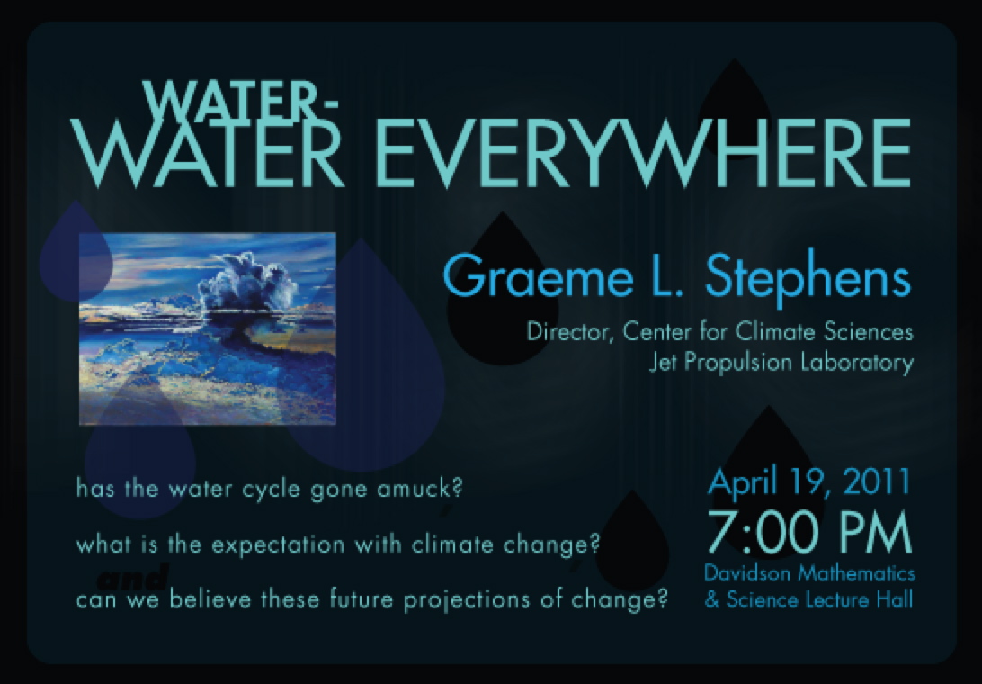
Extra credit seminar for Tuesday night, April 19th.
Likely topic at seminar: Satellite remote sensing to
improve our knowledge of the Earth's energy budget.
Reno's Peavine mountain and the pilot's bow (glory) in the cloud.
ANNOUNCEMENT: UNR American Meteorological Society meeting. When: 6:00 pm Thursday April 7th. Where: Leifson Physics Conference RM, 2nd floor of the building. Subject: Introduction to tropical meteorology and meteorology of Costa Rica. Presenter: Marce Loria, UNR Atmospheric Sciences Grad Studen. All are welcome to attend! Dinner will be served.
Time Lapse Video of clouds on the night of 3 April 2011 from Reno looking east.
Public lectures on Thursday the 7th. 6 pm at Leifson Physics RM 213 INTRODUCTION TO TROPICAL METEOROLOGY AND THE WEATHER IN COSTA RICA by Marce Loria, UNR Grad Student. Also,
Week 10: 28 March - 1 April. Print out the skew T log P diagram and prepare to use it for class.
Chapters 6. Presentation. Notebook complete up through chapter 5 is due on Wednesday. Chapters 3, 4, and 5 will be graded this time.
DEMONSTRATIONS:
Prepare a rubber stopper with a tube through the center. Place the stopper on a 2 liter clear plastic soda bottle filled 3/4 with water. Pump the air up inside the bottle... suddenly the stopper is blown off. A cloud forms inside the bottle. Here is what happened. As you pump up the air pressure inside the bottle the compression naturally heats the air, though because you are pumping it up slow, the heat travels from the pump and the bottle to the surrounding room air very effectively, as well as to the water in the bottle. Then suddenly the cork flies off the bottle (be careful to protect your eyes). The air pressure drops by about a factor of 2 very suddenly and so the air inside the bottle is cooled rapidly, so much so that the air temperature drops to the dew point and cloud forms. It is particularly effective to use an 'elmo' presenter pointed at the bottle and to project the image overhead.
Demonstrate diffraction by using a laser pointer, a business card, a single strand of hair, a pocket knife, and some scotch tape. Cut a square hole in the business card, about 2 cm on a side (about 1 inch). Tape the hair to span the middle of the card freely (put the tape on the remaining part of the business card.) Shine the laser through the hair to a distant screen in a dark room. Diffraction fringes will appear, much like the diffraction that happens when sunlight (direct or reflected from the moon) is diffracted by thin water droplet containing clouds when single scattering dominates and when particle size distribution is fairly monodisperse. This is the explanation for corona (not the beer, the colorful rings around the moon or sun) and cloud irridescence. The location of the maxima and minima in the diffraction pattern depends on hair size and wavelength, so it is a convenient way to use light to measure hair thickness. This demonstration is dramatic in a lecture hall when you can display the diffraction pattern on the ceiling or wall in a large room, and if the room can be made really dark.
Solar corona from Wikipedia. Click on image for a larger version.
Cloud iridescence on the wave cloud over Reno NV looking north during Fall 2010 atms 411 course. Photo by me. Click on image for a larger version.
Week 8: 7 March - 11 March.IF YOU ARE SICK, JOIN US AT THE ONLINE CLASSROOM AT THE REGULAR TIME! Those at home, print out the skew T log P diagram and prepare to use it for class.
Chapters 4 and 5. Presentations. For chapter 4, see especially the maps of RH and temperature for the presentation today.
Key Concepts: Atmospheric humidity. Condensation, dew, fog, and clouds.
Practice with the humidity calculator. Refer to the homework for chapter 4.
Read chapter 5. "When the dew is on the grass, rain will never come to pass. When grass is dry at morning light, look for rain before the night." Is this folk saying true for Reno summers?
Demonstrations: Skew T log P diagram from textbook, and as a gif file.
Important Example: Clash of hot dry air from the southwest with
warm moist air from the southeast: Dry lines and severe weather. (Image from Wikipedia.)
(Use skew T Log P or cross sections to demonstrate the complex vertical structure near the dry line.) Ship tracks in the ocean due to large amounts of air pollution from ships can be viewed in this presentation.
Chapters 4 and 5. Presentations.
Key Concepts: Atmospheric humidity (aka water vapor). Condensation, dew, fog, and clouds.
Prepare for class by reading chapters 4 and 5. Chapter 4 will largely be discussed on Monday, and Chapter 5 on Wednesday.
Read about water here too.
Absolute humidity, e = number of water vapor molecules per volume. Expressed commonly as the partial pressure due to water vapor, with symbol e. Can have any value from 0 mb to es, the saturation vapor pressure described next, (and maybe a bit more than es in clouds.)
Saturation vapor pressure, es = partial pressure of water vapor at saturation above a surface of liquid water at temperature T. Symbol es. It only depends on temperature. Has a value of 2.4 mb at -10 C, and a value of 70 mb at 40 C. It increases rapidly with increasing temperature.
Relative Humidity, RH = 100 * e / es. It is the ratio of the vapor pressure e to the saturation vapor pressure es. It is the humidity present relative to the humidity that would be present at saturation in an environment where the temperature is T. Values normally are in the range from 0 to 100%, though values larger than 100% are possible when 'super saturation' occurs like in clouds.
Dew Point Temperature Tdew = temperature air must be cooled to for condensation to start forming on things. The range of values can be from 0 Kelvin (absolutely dry conditions with no water vapor) to the environmental temperature T. Calculate values of Tdew from T and RH values.
Mixing Ratio, w = Mass of water vapor in a given volume / Mass of dry air that is in that same volume. Typical units are grams/kilogram, and they are expressed that way so that typical values for room air temperature might be values of 2 g/kg or 20 g/kg, depending on the relative humidity. Use the humidity calculator here.
Wet bulb temperature Tw = The temperature air can be cooled to by evaporating water into it. It is the temperature of air that comes out of a well functioning 'swamp cooler' also known as an evaporative cooler, a type of air conditioner to provide comfortably cool air in dry climates on hot days. Tw is greater than Tdew, and is less than the environmental temperature T. It is the temperature you feel when your skin is wet and is exposed to moving air.
Demonstrations:
Use the humidity calculator to explore a number of features of water vapor, like air density dependence on water vapor concentration.
What happens when you see your breath?
We used the thermocouple temperature gauge to measure room temperature and wet bulb temperature.
Then we went to the look up table and obtained the dew point temperature and relative humidity.
Then we used the skew T Log P plots for the first time to find the wet bulb temperature from the dew point temperature and air temperature.
We also discussed the dry adiabatic lapse rate, and the lifting condensation level and how they are read from the skew T log P plots.
Students used laminated skew T Lop P plots with dry erase markers to put on points and simulate the atmosphere thermodynamics.
What's wrong with this picture?
Space shuttle view. Click for larger image. Space shuttle launch
GOESSatellite loop on 26 Feb showing orographic forcing and a 'fire hose' delivery. (Geostationary satellite.)
Week 6: 21 February - 25 February.
Weather pattern during our snow storm last week.
Check out the massive mesoscale system north of Hawaii.
IT IS NOT ACCEPTABLE TO BRING YOUR LAPTOP TO CLASS AND PLAY GAMES. IT DISTRACTS ME AND OTHERS. PEOPLE PAY GOOD MONEY FOR COURSES, AND THOSE FEW OF YOU WHO LOUDLY PLAY GAMES ARE MESSING IT UP FOR EVERYONE. THIS IS TOTALLY UNACCEPTABLE BEHAVIOUR IN THE CLASS ROOM. QUIT DOING THAT!!!! FROM NOW ON, RATHER THAN DISRUPT EVERYONE, REDEEM YOURSELVES BY SITTING IN THE FRONT ROW, FAR APART FROM EACH OTHER, PAY ATTENTION, BE QUIET, AND PARTICIPATE IN THE CLASS, AS DO OTHERS. THIS IS AN AWESOME CLASS!!! LET'S ALL WORK TOGETHER TO MAKE IT THE BEST IT CAN BE FOR ALL, AND MAKE THE LEARNING ENVIRONMENT WORK FOR EVERYONE.
Chapter 3 presentation. Work on homework for chapter 3. Due date moved to Monday 28 February.
Continue to discuss temperature variations in the planet: The reasons for the seasons!
Demonstrations:
Class on February 16th was devoted to understanding 'the reasons for the seasons'; that overhead sunlight produces more intense heating at a spot on the surface than does sunlight arriving at large zenith angle near sunset or sunrise. An Ocean Optics Optical spectrometer was used to observe the spectrum of light from the fluorescent lights overhead (atomic emissions from mercury) with applications to understanding how spectral analysis can be used to study composition; then a heat lamp was used with an infrared thermometer to heat dark surfaces. The heat lamp also was used to enlarge a plastic water bottle partly filled with dark ink so as to strongly absorb light (this is the example of how a green house works: It is NOT the example of how the so-called 'greenhouse' effect in the atmosphere works. The atmosphere is NOT like a greenhouse. The greenhouse warms because hot air from absorbed solar radiation can not leave the greenhouse to be replaced by cooler air. In the atmosphere, warming is caused by emission of infrared radiation from the atmosphere to the earth's surface where the IR is absorbed and heats the surface). We observed the spectrum of the heat lamp too and noted that the peak of the spectrum (650 nm) was at a longer wavelength than the solar peak
(500ish nm) because the heat lamp is not as hot at the sun. Then we measured the spectrum of an incandescent flash light, a 'white' LED (turns out it was blueish as noted in the spectrum as well), and a laser diode laser pointer. We briefly discussed the difference between a light emitting diode and a laser diode (optical cavity in the latter case), and how the green laser points are made (808 nm laser diode drives a NdYAG crystal into oscillation at 1064 nm; nonlinear optics doubling of that light to 532 nm by another crystal). A brief discussion of the eventual appearance of green laser diodes, and the miniature laser diode based projectors that will come about as a consequence was entertained. Then the 'thumb and fist' earth with its rotation axis was used to simulate the path of the Earth around the sun with the relationship of seasons coming about from the relative tilt of the earth to the sun.
Idea: Latent heat, the hidden heat, the heat absorbed or released during a change of phase, during water condensation, evaporation, melting and sublimation.
Demonstrations: Blue sky, red sunsets, Rayleigh scattering by particles or molecules much smaller than the wavelength of light, multiple scattering, polarization of light by Rayleigh scatterers.
Need: flashlight, preferably a decent 'spotlight' type of flashlight with a nice white light source. A clear glass tall enough for all in the class to see. A polarizer. A small carton of milk to use to simulate clouds. Shine the flashlight through the cup filled with water. Use the polarizers at each step by putting it in between the glass and the audience, and rotating the polarization to illustrate the polarization by Rayleigh scatterers after a few drops of milk are added to the cup. Notice that the 'white' milk looks 'blue' in the cup after it is added to the water in a very diluted state. Note that the light scattered towards the audience is enriched in bue color, and the light passing straight through a white screen or wall is enriched in red color (Rayleigh scattering, or scattering of light by small particles, is much stronger for blue light than for red. Selective scattering makes the light red on transmission because the blue has been scattered away.) As more milk is added the intensity of color becomes greater, though polarization on rotation diminishes as multiple scattering in the more concentrated water/milk mixture. Eventually with enough milk added the water is back to 'white' looking as multiple scattering (light entering the glass scatters off of many milk particles before leaving the glass) is homogenized by multiple scattering.
Eye color is strongly affected by Rayleigh scattering and by the amount of light absorbing melanin in the iris. Return.
Keep in mind: homework from chapter 2 is due on Wednesday. Bring clickers to class for Wednesday 9 February 2011 class, and from now on. We'll start using them on Wednesday.
Chapter 2 . Read chapter 2 in preparation. The focus of this chapter is on the energy pathways and balance in the atmosphere, as well as a discussion of 'greenhouse' effects (the dance between radiation partners, solar and terrestrial light, and absorbers like the infrared active gases in the atmosphere and the Earth's variable surface.)
Here we also consider the explanation of the blue sky!
Finish lecture on chapter 1. Chapter 1 homework due on Monday.
Begin chapter 2. Read chapter 2 in preparation. The focus of this chapter is on the energy pathways and balance in the atmosphere, as well as a discussion of 'greenhouse' effects (the dance between radiation partners, solar and terrestrial light, and absorbers like the infrared active gases in the atmosphere and the Earth's variable surface.)
Week 2: 24 - 28 January
Finish reading chapter 1. Work on the homework for this chapter.
Plan on attending one of the sessions with a TA as discussed in class on Monday the 24th.
Chapter 1 presentation. Earth's radius is about 6371 km. Compare that with the height of the atmosphere, maybe 100 km.
1. Students often confuse water vapor with liquid water. Students should understand that water vapor is an invisible gas. Haze, fog, clouds, and the steam from a boiling pot all become visible when water vapor condenses and forms small drops of liquid water. This can be easily demonstrated using a tea kettle, or by showing a video of water boiling in a tea kettle.
2. The introductory explanations of the air motions associated with high and low pressure centers and fronts make this a good place to begin to show and discuss satellite photographs, loops, and surface weather maps. Many students have occasion to watch television weather broadcasts. Being able to observe and understand weather phenomena on their own may heighten interest in the subject. Download a few satellite loops off the Internet and discuss the air motions.
3. Speculate on how we know the chemical composition of the earth's early atmosphere
Additional extra credit ideas for your notebook in addition to the required "Questions for Review":
B. Carry your cloud identification chart from your text book around with you. Take photographs of clouds yourself, and identify the time and date they occurred. Put these photographs and a brief discussion of them in your notebook too.
Awesome examples of clouds associated with Kelvin Helmholtz wind shear instability in the atmosphere. Note how they look like waves breaking on the ocean. Photos taken by Laurie Arnott-Klausner on December 10, 2010, late in the morning, looking west towards the Wet mountains, west of Pueblo CO, from the foothills of the Wet mountains, just south of HW96.
KH Wave cloud broad view (click on image to see larger size)
KH Wave cloud close up view
Broad NASA Aqua Satellite view from December 10th.
Introductions. Syllabus. Read chapter 1. We did to demonstrations as follows:
1. Fill a wine glass completely with water and cover it with a piece of plastic (such as the lid from a tub of margarine), being careful to remove any air. Invert the glass. The water remains in the glass because the upward force on the cover due to the pressure of the air is much stronger than the downward gravitational force on the water.
2. Place a candle in the center of a dish and partly fill the dish with water. Light the candle and then cover it with a large jar or beaker. The flame will consume the oxygen inside the jar and reduce the pressure. Water will slowly flow into the jar to re-establish pressure balance. The change in volume will be close to 20 percent, the volume originally occupied by the oxygen in the air. This demonstration can be used to illustrate the concept of partial pressure, which is later used in the chapter on humidity. The students should also be asked what they think the products of the combustion might be and why these gases do not replace the oxygen and maintain the original pressure in jar. One of the combustion products is water vapor, which condenses as the air in the jar cools. Another combustion product is carbon dioxide, which presumably goes into solution.


