

ATMS 748 Homework and Course
Deliverables (return to main page)
[How to write lab report]
Purpose:
Learn about typical and anomalous air quality and meteorology in Reno/UNR for February 2020.
Work with raw data to get a feel for time alignment issues, and use of Excel data base functions for making Diel averages (24 hour averages).
Learn how to do a case study for diagnosing and understanding specific events.
Learn about and work with data from the sonic anemometer, low cost air quality sensor SPS30, and the BAM1020 instrument used for PM measurements in cities to regulate air quality.
Learn how to use HYSPLIT back trajectory analysis and Google Earth to determine likely source regions for windblown dust.
Learn about remote sensing with the Cimel and MFRSR sunphotometer and spectral irradiance for obtaining column aerosol optical depth (AOD), with an eye towards satellite remote sensing of AOD.
Learn how to use Python to make wind roses and air pollution roses.
Discussion:
This assignment is open ended in that we will work on it as a group, online and outside of class, and will consider as many learning experiences as possible with the time remaining this semester.
We routinely measure local and column properties of the atmosphere from the roof of
the Physics building, with standard and custom instruments of our own manufacture.
Reno also has the National Weather Service and many weather stations at various elevations.
Our unique location
results in brilliantly clear days, inversions with air quality issues, and days with windblown dust arriving from nearby dry lake beds.
Notes:
Please be sure to reach out to me during online class or afterwards if you are having issues.
We will make sure everyone is caught up and complete in working through this assignment.
Feel free to share your skills and expertise with the everyone.
Deliverables:
1. A report with references, as we have been doing all semester. See below for report contents.
2.
A presentation containing your specific case study. See below for details.
Required and Recommended Software:
1. Zoom online class interface. Here's the link for our class.
2. Excel and Word. Available for students and faculty here. Sign in with your UNR netID and download Office to your computer. We will import data using the text wizard: Excel:File:Options, then check this box.
3. Google Earth available here.
4.
Anaconda distribution of Python available here. We will likely use 'Spider' to edit and run Python programs.
5. You can use Matlab or any other program if you want, for data and graphical analysis.
|
|
|
 |
 Broad view of the sonic anemometer and others. |
 Close up of the sonic anemometer. |
| Documentation: Sonic anemometer manual. Presentation 1, Presention 2, Presentations 3. Gill manufacturer of sonic anemometers. RD Young manufacturer of sonic anemometers. |
Data for February 2020: |
 Beta Attenuation Monitor (BAM) Inlets for PM2.5 and PM10. PM2.5 has a cyclone to remove aerosol larger than 2.5 microns in diameter. (Article on cyclones). |
 How a cyclone works to take out larger aerosol by impaction and vortex flow. From this article on bioaerosol detection. |
 The two BAM instruments at UNR, inside the telescope dome. |
|
 Detailed view of the radioactive C14 source for the BAM detection scheme. |
|
Documentation: Calculate the speed of 49 KV electrons from the radioactive source. |
BAM Data for February 2020: BAM Zero Filter Data for 7-12 November 2019: HOURLY MEASUREMENTS: |
 SPS 30 mounted near the photoacoustic instrument inlet on the 4th floor of Leifson Physics roof area. |
|
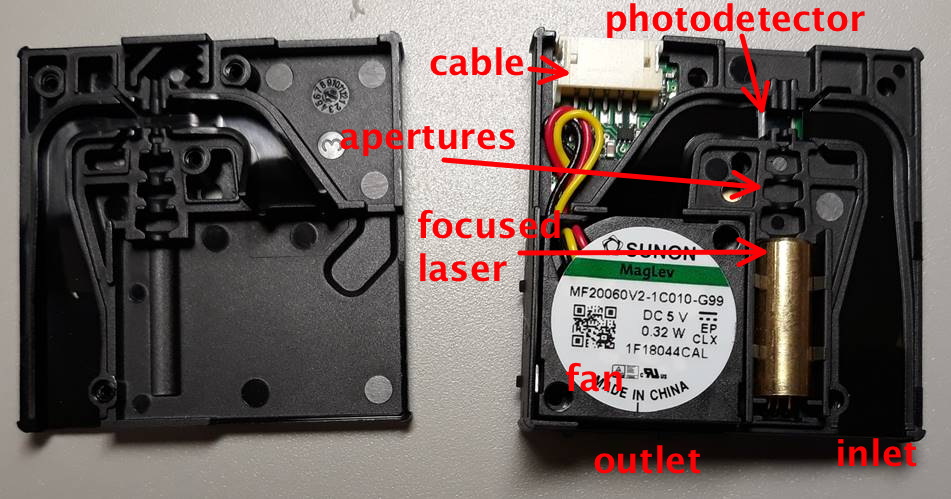 Detailed view of the interior of the SPS30 particle sensor. |
MINUTE MEASUREMENTS INCLUDE: a. Aerosol size distribution from 0.3 um to 10 um in 5 bins. b. PM1, PM2.5, PM4, and PM10. c. Ambient temperature and relative humidity. PROPERTIES CALCULATED FROM THE SIZE DISTRIBUTION MEASUREMENTS: a. PM1, PM2.5, and PM10 (to evaluate reported values). b. Aerosol light scattering coefficient, and asymmetry parameter at 19 wavelengths from the UV to the near IR assuming spherical particles, for PM1, PM2.5, and PM10 size cuts. |
Documentation: |
SPS30 Data for February 2020: |
 Blow up of the MFRSR, from the MFRSR Manual. |
 View of the MFRSR mounted on the roof of the Physics building. It is vital that the diffuser is horizontal, and that the motor points due to geographic north. |
|
 MFRSR electronics/control box. (Old school but effective.) |
| Documentation: MFRSR Handbook. Manuscript describing measurements from the MFRSR. |
MFRSR DATA FOR FEBRUARY 2020: |
 |
|
| Documentation: Video of the sunphotometer in operation. Sunphotometer presentation by Chris. Aeronet network description. |
Cimel Data Portal: |
Summary of Data For February 2020:
Sonic anemometer data. (right click and save link as a file on your computer).
Beta Attenuation Monitor (BAM). Right click on link and save it to disk.
SPS30 Low Cost Air Quality Sensor. Right click on link and save.
MFRSR Total, diffuse, and direct; and aerosol optical thickness retrievals.
UNR Cimel Sunphotometer data portal.
Meteorological Soundings from the Reno NWS, February 2020.
Resources and References:
In situ light scattering and absorption theory and measurements:
Light scattering by wind blown dust.
Photoacoustic instrument manual for aerosol light scattering and absorption measurements.
Photoacoustic optical properties at UV, VIS, and near IR wavelengths for laboratory generated and winter time ambient urban aerosols.
Sonic Anemometer:
Sonic anemometer manual.
Presentations on sonic theory and student projects. Presentation 1, Presention 2, Presentations 3.
Gill manufacturer of sonic anemometers.
RD Young manufacturer of sonic anemometers.
Beta Attenuation Monitor (BAM1020):
BAM1020 Manual.
How a cyclone works to take out larger aerosol by impaction and vortex flow. From this article on bioaerosol detection.
Calculate the speed of 49 KV electrons from the radioactive source.
About radioactive decay.
SPS30 Low Cost Air Quality Sensor:
Data sheet describing the SPS30
How to install the SPS30
Article on performance of low cost air quality sensors, including the SPS30.
Our website with SPS30 software
Article discussing 'machine learning' to improve the response to PM Coarse aerosol.
MFRSR Remote Sensing Instrument
MFRSR handbook.
Manuscript on MFRSR measurements.
Sunphotometer theory for remotely sensing column aerosol optical depth.
Sun photometer theory.
Our sunphotometer analysis website (air mass and Rayleigh optical depth calculator based on Perl language, here's the source code).
Articles describing aerosol and health.
Dissertation (see Figure 6).
Journal article (see Figure 2).
Related References:
Satellite Remote Sensing of Particulate Pollution from Space: Have We Reached the Promised Land?
Combine the ideas of the next two papers
to estimate potential hygroscopic growth of aerosol based on RH and aerosol chemistry.
Accuracy of near surface aerosol extinction determined from columnar aerosol optical depth measurements in Reno, NV, USA, especially Fig 4.
Revised Algorithm for Estimating Light Extinction from IMPROVE Particle Speciation Data
Photoacoustic analysis of combustion aerosol presentation, including a world tour.
Meteorological Soundings from the Reno NWS, February 2020.
Air pollution and meteorology in Russia: similar to our case study.
Mexico City aerosol 2009 paper.
Mexico City and Queretaro 2019 paper.
Per capita air pollution paper.
Reno winter time air pollution paper.
Hysplit air trajectory model.
Applications of air trajectory analysis review article.
Infrared radiation model for clear skies, and calculation of cloud effect.
Beijing fine and coarse mode aerosol composition.
Read in sonic data, and SPS30 data to an Excel spreadsheet.
Make a time and date column for each data set as the sum of the separate time and date columns.
Time align the data (get rid of data with time stamps on the same for both. Sometimes there is missing data).
Calculate the wind speed and direction from the sonic data. (Note the directions used for the sonic anemometer). Wind Direction=ATAN2(-E2,-D2)*180/PI()+180, Wind Speed==SQRT(E2^2+D2^2)/10, D2 is U; E2 is V.
Make a time series graph of
SPS30 PM2.5 and overlay BAM PM2.5. Note the high and low values of PM2.5. Note the level of agreement of disagreement of PM2.5 by these instruments.
Make a time series graph of
SPS30 PM10 and overlay BAM PM10. Note the high and low values of PM10. Note the level of agreement of disagreement of PM10 by these instruments.
Make a scatter plot of SPS30 PM2.5
on the y axis, and sonic wind speed on the x axis. Does wind speed seem to predict PM2.5 levels?
Make wind roses and air pollution roses using Python code, using Spyder and Anaconda, here's example data. What direction does most of the wind come from as a function of wind speed? What direction does most of the aerosol pollution come from.
Perform diel averages [and standard deviations in box and whisker format] (typical 24 hour day in Reno) for [overlay wind speed, kinetic energy, turbulent kinetic energy,] [overlay sonic temperature, pressure,] [overlay SPS30 pm2.5, SPS30 PM10, BAM PM2.5, BAM PM10.]
[overlay is to put these on the same graph].
Make a time series bubble graph of wind direction for Feb 8th. Make bubble size the wind speed to understand when the wind is greatest and lowest, and what direction it is coming from.
Make a time series bubble graph of wind direction for Feb 8th. Make bubble size PM2.5 to understand when the air pollution is greatest and lowest, and what direction it is coming from.
Get the Cimel AOD graph for the 8th, and any retrieved size distributions to see if there is a correspondence with PM2.5.
Get the MFRSR AOD graph and radiation graphs to get a sense of cloudiness for this day and time, and the effect of aerosol on total and diffuse radiation.
Find the time of peak PM2.5. Do Hysplit back trajectory analysis to the Physics building roof (about 25 meters above ground level) to find out where the aerosol was likely coming from for this day/peak.
Use Google Earth for displaying back trajectories and see if they 'explain' where the aerosol came from. Building coordinates are Latitude= 39.540980° Longitude=-119.814090° .
Hysplit air trajectory model presentation.
Applications of air trajectory analysis review article.
Repeat the steps in part b for another day of interest.
You could choose a really clean time, or polluted time, on a different day, to see if you can interpret the aerosol pollution or lack thereof.
1. Is the surface aerosol size and composition affected by updrafts and downdrafts at the surface and in the column?
Associated questions:
a. Are their persistent and strong updrafts and downdrafts at our site? (use the vertical component of wind from the sonic anemometer to answer this question.)
b. What time of day are they most noticed?
c. How do clouds affect the presence of updrafts and downdrafts?
INSTRUMENTS
i. SPS30 aerosol sensor especially for PM2.5 (4 seconds and 1 minute) Surface temperature, dewpoint, and RH (4 seconds and 1 minute)
ii. Sonic anemometer on the roof (5 Hz and 1 minute)
iii. MFRSR Solar spectral solar irradiance with shadowband for direct and diffuse radiation.
2. Can the surface PM2.5, PM10, and PMCOARSE (PM10-PM2.5) be 'explained' by surface meteorological conditions, wind speed, direction, temperature, humidity, pressure, at the surface and boundary layer height determination?
Associated Questions
a. Does the SPS30 PM2.5 and PM10 agree with the Beta Attenuation (BAM) hourly PM2.5, PM10, and PMCOARSE well enough that we can use them interchangeably? (so far we see that PM2.5 is ok).
The SPS30 has 4 second data while the BAM data is hourly. It's useful to have fast measurements but only if they are actually reasonable.
INSTRUMENTS
i. BAM1020 Beta Attenuation instrument
ii. SPS30 PM sensor
iii. National Weather Service Balloon soundings (boundary layer height, time/height graphs of column relative humidity, and aerosol hygroscopic growth dependent on aerosol chemistry).
PARTIAL LIST OF REFERENCES (student can find others)
Black carbon aerosol concentration in five cities and its scaling with city population.
Photoacoustic optical properties at UV, VIS, and near IR wavelengths for laboratory generated and winter time ambient urban aerosols.
See figure 4 of Accuracy of near surface aerosol extinction determined from columnar aerosol optical depth measurements in Reno, NV, USA.
3. Is the surface aerosol optical properties measured with photoacoustic instruments and their nephelometers 'the same as' the column optical properties?
This is a central assumption of using satellite remotely sensed aerosol optical depth for surface aerosol pollution determination.
Associated Questions
Can the column aerosol optical depth be used with the surface extinction coefficient to obtain the atmospheric boundary layer height?
INSTRUMENTS
i. Cimel sunphotometer level 1.5 data (cloud screened)
ii. MFRSR aerosol optical depth measurements
iii. 405 nm photoacoustic instrument data averaged to 30 minutes or ?
iv. 532 nm photoacoustic instrument data similarly averaged.
v. Perhaps 660 nm data
vi. PAX 870 nm data as it becomes available.
iv. National Weather Service Balloon soundings (boundary layer height, time/height graphs of column relative humidity, and aerosol hygroscopic growth dependent on aerosol chemistry, and downwelling spectral IR based on the FASTCODE model).
PARTIAL LIST OF REFERENCES (student can find others)
Satellite Remote Sensing of Particulate Pollution from Space: Have We Reached the Promised Land?
Photoacoustic optical properties at UV, VIS, and near IR wavelengths for laboratory generated and winter time ambient urban aerosols.
Combine the ideas of the next two papers
to estimate potential hygroscopic growth of aerosol based on RH and aerosol chemistry.
Accuracy of near surface aerosol extinction determined from columnar aerosol optical depth measurements in Reno, NV, USA, especially Fig 4.
Revised Algorithm for Estimating Light Extinction from IMPROVE Particle Speciation Data
The goals of this assignment are:
a. Explore the use of LEDs and photodiodes as light detectors for applications as radiation detectors.
b. Introduce a very common, and extremely useful integrated circuit for electrical signal conditioning, the operational amplifier.
c. Reinforce how you can get quantitative measurements from the Arduino and/or Teensy boards.
d. Reinforce the difference between ideal voltmeters and real voltmeters, that meter input resistance matters
 By way of review, here's the photoresistor circuit we used in the past for measuring light. Click on the image for a larger version. |
A. We will replace the photoresistor with an LED, now with the LED being used as a wavelength selective detector in addition to as a light source.
Build a simple circuit with a resistor and LED as a photodetector so that you can measure the photocurrent from the LED such that 0.1 microamps produces a 1 volt signal.
See the schematic diagram below.
You can use the modified sketch for the photoresistor response time measurement, and CoolTerm for this lab too.
Adjust 'jmax' to see the effect of signal averaging on the noise reduction.
Record and graph the waveform for the LED as a detector with the output of the LED being measured as the voltage across the resistor.
 Notes for the lab. Part A refers to the left, and those with the opamps to the second part. Click on image for larger version. |
 Schematic for these measurements. Here's the ExpressPCB file. |
 We will set up this circuit first. Click on image for larger version. Set this up on the Arduino using the schematic as a guide. |
 We will set this up second after the previous set up has been used. Photograph of the Arduino set up measurements with an opamp as a signal conditioner. Click on image for larger version. |
 Photograph of the Teensy 3.6 set up measurements with an opamp as a signal conditioner. Click on image for larger version. |
B. Construct a transimpedance amplifier circuit with an op amp to convert the photocurrent from the LED as a light detector to a voltage so that a photocurrent of 0.1 microamps produces a 1 volt signal.
Add a 4.7 pF capacitor in parallel to the feedback resistor to form a low pass circuit.
Make observations of this waveform as in part A.
Write your data to a file using CoolTerm.
Graph your time series. Compare the response time and noise of these circuits.
EXTRA CREDIT: C. Repeats parts A and B using the OSRAM BPW34 photodiode as a detector instead of the LED.
This detector is much more sensitive than an LED, so you may have to use much less LED light, and also a dark room (or cover up the circuit to shield it from room light.
 |
 |
EXTRA CREDIT D. (As time permits: extra credit). Set up the non inverting amplifier circuit with a feedback resistor of 2k Ohm and 2.2uF capacitor in parallel, with a resistor of R2=10 MegOhm.
Measure a pulse from the LED using the same Arduino program we used for testing the photoresistor.
Show the effectiveness of shielding the circuit with aluminum foil. Photograph of the set up, and example data.
E. Analysis for your report.
a. Present and compare pulse waveforms measured in parts A and B (and C and D if pursued).
b. Estimate the response time, τ, from your time series graph as shown in the figure below to obtain the response time of the resistor/LED circuits.
c.
Using part b, calculate the LED and photodiode capacitance, C, using τ=RC.
Extra credit for your write up.
d.
Discuss the operational amplifier 'golden rules' and derive the equation used to obtain the output voltage relationship with the light detector photocurrent for the circuit of part B.
e. Derive the equation for the low pass filter effect of the capacitor and resistor on the sensor response in part c.
 |
Discussion of operational amplifiers.
Input impedance of a transimpedance amplifier and local backup.
Photodiode technical information sheet.
OSRAM BPW34 photodiode data sheet.
PIN photodiode description relevant to the OSRAM photodiode. (local backup).
Photodiode FDS100 we typically use in our aerosol light scattering detectors.
Thorlabs site that nicely describes use of photodiodes to detect light.
Photodiode discussion.
Resistor and capacitor circuits in the time and frequency domains, and low pass filter response of an RC circuit. (local backup).
Assignment 2 Arduino, Teensy, and
Atmospheric Measurements:
This assignment will be submitted in 3 parts, see webCampus,
parts 1&2; parts 3&4; parts 5&6
Title: You can decide on the title based on your experience with
this lab.
Goals:
a. Become familiar with the Arduino
microcontroller as an example of a programmable device for acquiring
measurements and controlling systems.
b. Demonstrate ability to modify Arduino sketches for solving problems.
c. Learn about and use sensors with atmospheric relevance.
d. Learn how to bring measurements from the Arduino into computers
(interface the Arduino) to acquire data for later analysis and display.
If possible, install the Arduino
software on your own laptop (if you have one), and use it in class.
Also download CoolTerm and
place it somewhere that you can get to it for ease of use. This program
allows us to transfer data from the Arduino to the computer.
The code for the projects in the book and kit is here:
expand the file and put the folder in your Arduino examples folder.
Here is a link
to the an online version of a manual that is similar to the one we use
in class. (local backup).
In your report, describe and/or answer these questions
1. Introduction to describe the Arduino (why is everyone so crazy about
this thing?).
Then create a circuit to drive the LED at different frequencies to see if
the photoresistor resistance can accurately follow the LED output for low
and high frequencies.
Point the LED output directly into the photoresistor input. You can use
variable delay and the 'Blink' sketch to drive the LED to write your own code, or
here's an example sketch that does the calculation in Lux, read through it so you understand it.
 Description of the circuit for the photoresistor test. Click on the image for a larger version. |
If the LED is driven by a square wave, the photoresistance should show a
crisp square wave too. Use the plot monitor on Arduino to view the
photoresistor output,
and save some data with CoolTerm
(including time) so that you can graph the photoresistor output from the
LED drive as a function of time.
Obtain an approximate value for the time constant of the photoresistor as a sensor of
light from a graph of the data.
The light intensity is calculated using the equation LUX = 1.25*107*Rp-1.41 where Rpis the photoresistance in Ohms. (local backup of link).
Then work out the response time of the photoresistor for measuring light using the Solver within Excel.
As time permits, do one set of curves for room lights on, and another for lights off. Is there any difference in the time constant caused by spanning the photoresistor over such a large range of light intensity?
Be sure to photograph your setup and use it in your report.
Answer these questions in your write up.
What is the principle of operation of the TMP36 temperature sensor? How
was its signal obtained?
Obtain and discuss the time constant for the sensor as you are
warming it up with your fingers, and the time constant as you are
cooling it off by letting it sit in air.
First use the sketch for circuit 7 to view the measurement. Then proceed with the sketch mentioned below the figure.
Description of the analog to digital conversion for
the TMP36 sensor. Click on image for a larger version. |
Improved example sketch
for response time measurement. Read it and follow instructions.
Note especially the way that time averaging is implemented in the sketch with the function at the bottom of it, and the difference in this sketch compared with the one for circuit 7.
Pinch the
temperature sensor to warm it up when the LED comes on.
Record a time series with CoolTerm
as you pinch the the sensor to warm it up to a steady temperature, and let
it decay to a lower temperature.
Obtain and discuss the time constant for the sensor as you are warming it
up with your fingers, and the time constant as you are cooling it off by
letting it sit in air.
Presentation on the TMP36 temperature sensor principle of operation.
Answer these questions in your write up.
What is the principle of operation of the thermistor temperature sensor?
How was its signal obtained?
Obtain the response time for the sensor as you are warming it up with
your fingers, and the response time as you are cooling it off by letting
it sit in air.
You might also be able to put the board and sensor into the freezer or toaster oven (on low heat setting) and do the measurements for the response time that way.
Measure the diameter of the TMP sensor and the diameter of the
thermistor sensor, and estimate the ratio of the mass of each sensor
assuming they have the same density.
Also determine the ratio of the surface area of each sensor.
Calculate the ratio of the response time of the TMP36 sensor to that of
the thermistor sensor, one ratio each for heating and cooling.
Does the ratio of response times compare mosty closely with the surface
area ratio, or the mass ratio?
Calculate the temperature that corresponds to your measured resistance
using the equation
given here (thanks Alex).
Record a time series using CoolTerm
as you pinch the the sensor to warm it up to a steady temperature, and let
it decay to a lower temperature.
Obtain the time constant for the sensor as you are warming it up with your
fingers, and the time constant as you are cooling it off by letting it sit
in air.
Here's an example
sketch to use for the thermistor sensor evaluation. Read the sketch
for instructions on what to do.
Pinch the thermistor carefully (without affecting the wires) when the LED
is on.

Click on image for larger version.
Answer these questions in your write up:
How does the pressure sensor work?
Can you see measure the pressure difference between the lowest level you
can get it, and the highest level?
Is that pressure difference correct?
Is the pressure sensor properly temperature compensated?
Do appropriate data averaging so that you can easily tell the pressure
difference
between having the sensor on the desk, and having the sensor about 1 meter
higher or lower. Record data with CoolTerm
to demonstrate your results.
Here's an example
sketch for the pressure sensor. You'll have to comment out some
lines near the end to get only the pressure measurements to CoolTerm.
Do measurements with 1 second time average, holding the sensor down for 10
seconds, then up for 10 seconds.
Then modify the code to obtain 10 second time averages. Test by holding
the sensor low for 100 seconds, and high for 100 seconds.
Comment on the effects of additionally time averaging the data.

Click on image for larger version.
Note: It seems the 10 bit analog to digital (a/d) converter of the
Arduino would not be able to resolve a pressure difference of about 0.1 mb
associated with
1 meter height difference. 1 bit change in the a/d counts corresponds to a
voltage change of about 0.005 volts, and a pressure change of and about 1
mb pressure.
Dither
helps: the voltage source for the Arduino is noisy enough to cause around
50 mv or so of noise so that the a/d counts fluctuate to a useful average.
The example sketch for pressure averages the measurements of the pressure
sensor voltage and the voltage divider voltage about 1800 times for each
measurement.
Use of the voltage divider for the power supply voltage measurement is
necessary since the a/d range is 5 volts, and direct measurement might be
If you are ahead, you may add the digital pressure sensor to the sketch and breadboard layout and compare the analog and digital sensors.
Demonstrate a time series of temperature by moving your hand over the
temperature sensor quickly, using Labview or cool term by doing a screen
capture or other means.
Include a discussion of how the sensor works.
Those with laptops can take the IR sensor outside to get a time series of
infrared brightness temperature of various targets.
 Notes on the IR sensor: Click on image for larger version. |
Additional Resources:
Description of the Arduino and
some sensors we'll use.
Discussion of
microcontrollers in general.
TMP36 temperature sensor
data sheet.
Presentation on the TMP36 measurement principle.
Very useful voltage divider circuit to use for measuring sensors that
depend on resistance.

Click on image for larger view.
|
Useful Presentations Collected from Others that describe
the Arduino and uses. |
Assignment 1: Presentation on an Atmospheric Instrument
Purpose:
a. Become more familiar with atmospheric instruments important for your
research and/or interests.
b. Share that knowledge with others in class.
c. Become familiar with presenting instrument descriptions.
Your presentation should consider the following:
a. Why you are interested in this instrument.
A. Instrument description, what does it measure?
B. What is the operating principle of the instrument?
C. What sensor(s) are used for the measurements?
D. What is the measurement range and uncertainty?
E. What factors affect measurement accuracy?
F. What are the size, weight, and power use of the instrument?
G. How does the instrument store data?
H. Provide measurement examples.
I. How is the instrument calibrated?
J. Provide other pertinent information.
K. How do the results from this instrument compare with others?
L. References
Action Plan:
Choose an instrument and ok it with the instructor (DOE
ARM Site suite of instruments provide a good list of current instruments).
Instrument Manufacturers and other links:
Apogee
instruments.
Vaisala.
Campbell.
Droplet Measurement
Technologies.
Spec Inc.
Yankee.
Comparison
of instrument for precipitation type discrimination. (from here).
Helpful MetEd Modules on Atmospheric Instrumentation:
Radar
Meteorology
Overview
of Instrumentation
Temperature
Measurement
| Student | Topic |
| Em | Ka band radar |
| Sam | ARM AERI (and FTIR) |
| Christopher | ARM CSPOT. Cimel sunphotometer and the AERONET network. |
| Sean | RADIOSONDES |
| Samantha | Active fire detection using MODIS (MCD14DL) |
| Courtney | Dopper Lidar |
| Mikhail | Ice detector |
| Stormi | FLASH B, FLuorescenst Advanced Stratospheric Hygrometer for Balloon, instrument |
| Matthew | Raman Lidar |


 SPS 30 sensor in my office used for indoor air quality measurements.