
Week 10: 26 October
Monday - Thursday
Continue to work on HW5.
Spatial scale of tornados and radar images.
Demonstration of polarization of light.
Use of the correlation coefficient and Doppler shift in identifying features of storms.
Chapter 3 presentation.
Week 9: 19 October
Thursday
Earth school approach for reanalysis after March 2026. See homework 5, part E for further instructions. (try also, https://climexp.knmi.nl/)
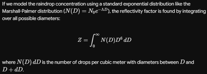
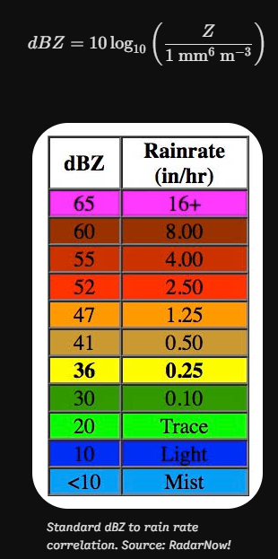
Of Rain and Radar... Z and dBz and interpretation.
Monday - Wednesday
Chapter 3 presentation.
Trapped lee waves downwind of the Sierras during windy events. A major application of buoyancy to a phenomena often observed in Reno and downwind of the Sierra Nevada Mountains.
Sound and radar propagation in the atmosphere, organized as a general wave phenomena governed by Snell's law. One Notes in addition to chapter 3 presentation.
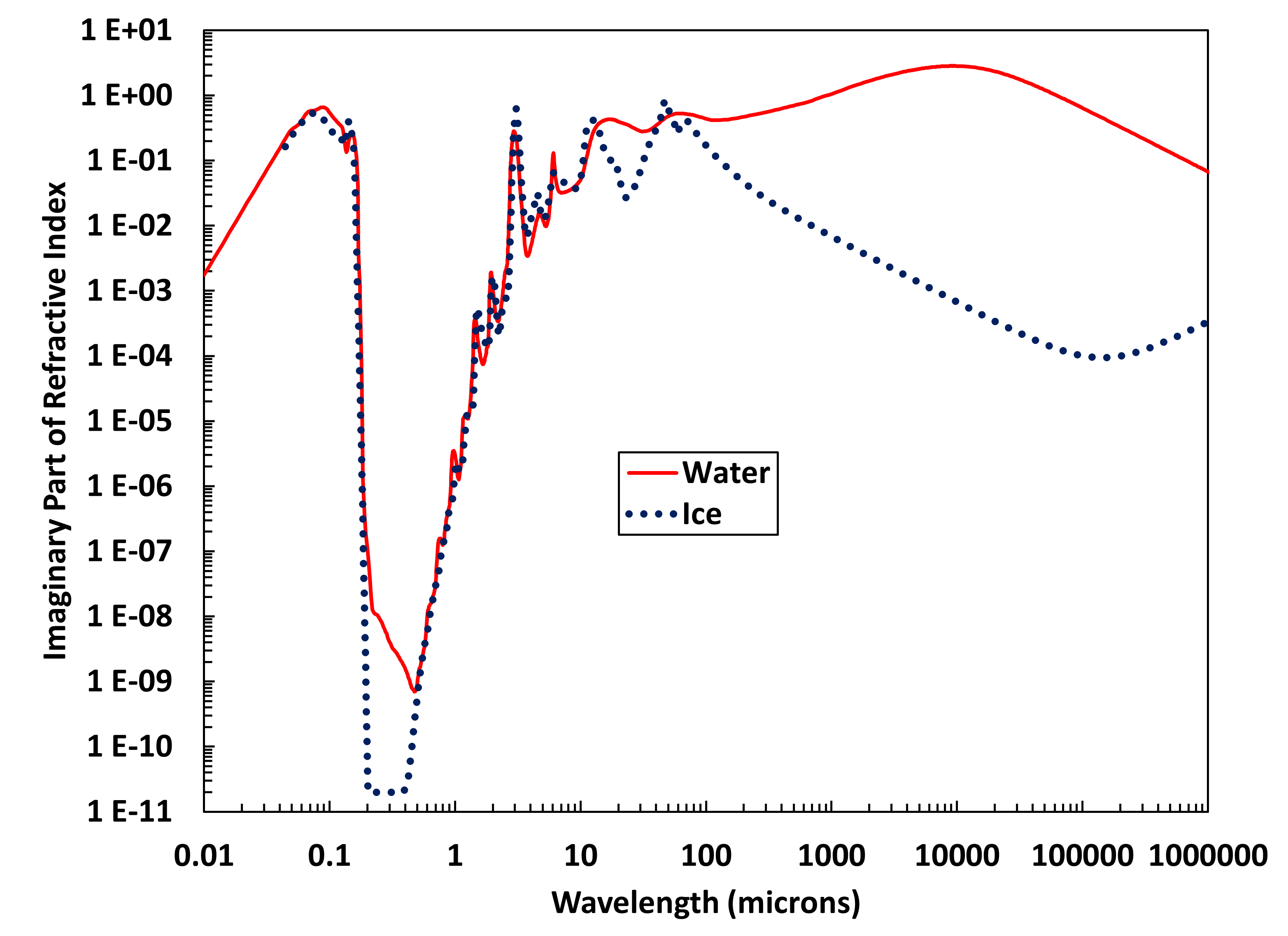
Real and Imaginary parts of refractive index for water and ice as a function of wavelength (spreadsheet containing values).
Classic book on light scattering by small particles like smoke.
Clouds in our area.
Amsterdam island, gravity waves.
Guadalupe island, vortex street.
Week 8: 12 October
Monday - Thursday
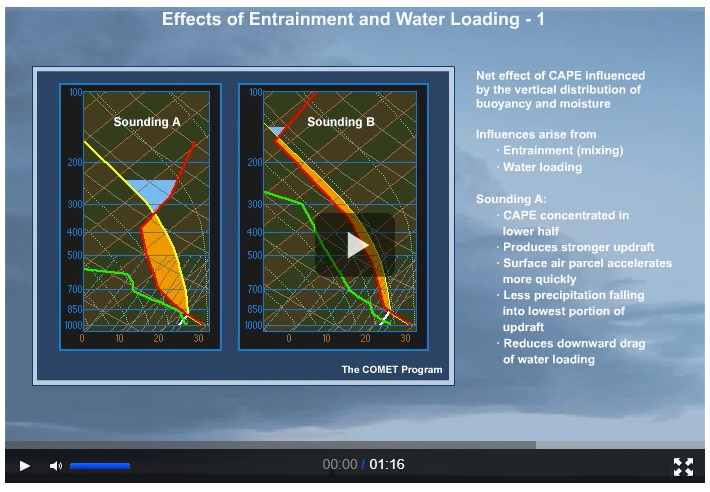
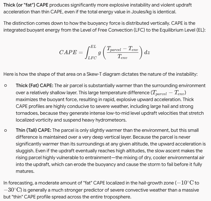
Of thick or thin CAPE as discussed in MetEd?
Gemini AI weighs in....
Wednesday and Thursday Examples:
Model soundings and vertical cross sections (Tropical Tidbits).
Wind flow over a mountain range and drying out of air mass.
Reno morning and afternoon soundings and stability in terms of the vertical distribution of potential temperature.
Lab: Nucleation of water cloud by adiabatic expansion.
Nucleation of ice cloud by adiabatic expansion in the freezer.
Crush can with water vapor and atmospheric pressure.
Tuesday: Quiz on adiabatic processes and potential temperature.
Geostationary lightning mapper satellite imagery.
NOAA's hurricane division and description of hurricanes.
Bring questions to class about hurricane theory for HW 4.
Read HW 5, CAPE and severe storms, and find a case study (wild-fire pyrocumulonimbus and/or firenado; tornado; derecho; hurricane),
To create a recent model sounding using HRRR, start at the Continental US scale and click on any point. This will bring up a sounding. Choose where radar indicates active precipitation, and compare with another elsewhere. Notice the Dendrite Grow Zone (DGR) elevations and associated temperatures.
Demonstrate ice crystal growth from supercooled water droplets in RM 113 freezer (measure freezer temperature).
Week 7: 5 October
Monday - Thursday
Review the surface pressure variation from day to day in Reno and comparison with the theory of pressure tides paper.
Theory of pressure tide script.
Freezing of water droplets containing salts. (See Chapter 6 presentation for details of cloud microphysics).
https://journals.aps.org/prl/abstract/10.1103/PhysRevLett.118.084101 article on this subject.
Geostationary lightning mapper satellite imagery.
Prepare hurricane theory for HW 4.
Read HW 5, CAPE and severe storms, and find a case study (wild-fire pyrocumulonimbus and/or firenado; tornado; derecho; hurricane),
To create a recent model sounding using HRRR, start at the Continental US scale and click on any point. This will bring up a sounding. Choose where radar indicates active precipitation, and compare with another elsewhere. Notice the Dendrite Grow Zone (DGR) elevations and associated temperatures.
Demonstrate ice crystal growth from supercooled water droplets in RM 113 freezer (measure freezer temperature).
Week 6: 28 Sept
Monday - Thursday
Obtain T and Tw outside for HW4 on Thursday.
Presentations finish for HW3, comparison of Rochambeau and Barrow.
Read HW 5, CAPE and severe storms, and find a case study (wild-fire pyrocumulonimbus and/or firenado, tornado, derecho, hurricane),
To create a recent model sounding using HRRR, start at the Continental US scale and click on any point. This will bring up a sounding. Choose where radar indicates active precipitation, and compare with another elsewhere. Notice the Dendrite Grow Zone (DGR) elevations and associated temperatures.
Week 5: 21 Sept
Wednesday and Thursday
Last problem in HW3 discussion. Presentations begin on Thursday.
Eliza, Sean, and Graham.
Solar radiation geometrical effects, inverse square law related to the elliptical orbit.
SOLPOS calculator settings for this problem.
Pressure from GPS discussion (Vaisala).
Tuesday
Work on HW3 in class. Python tutorial. Bring a laptop to class if you have one.
I will demonstrate how to use Colab as well. Prepare by getting a Google account if you don't have one.
Actions within Colab:
1. Create a new folder.
2. ! wget https://www.patarnott.com/atms401/HW3_Roch_Barrow2026.py (USE SHIFT ENTER TO EXECUTE THIS AND LINES BELOW.)
3. ! pip install metpy
4. ! pip install siphon
5. ! python
HW3_Roch_Barrow2026.py
Colab gives us full access to a Bash shell (among other things).
Our goal will be to have everyone get the data they need for HW3.
The program 'Spyder' within Anaconda can be used to run this script also. (Installer).
I will demonstrate Spyder as a second means of running this script.
(For reference, here's the discussion that was used with Gemini to obtain the script).
Last problem in HW3 discussion.
Solar radiation geometrical effects, inverse square law related to the elliptical orbit.
SOLPOS calculator settings for this problem.
Monday
Preparing for HW3 talks on Thursday (or earlier if ready).
How much water would it take to have a pressure equal to that of the entire atmosphere? (10 meters or about 33 feet).
Watch this video on Atmospheric Rivers.
Atmospheric river discussion.
Week 4: 14 Sept
Thursday
3. How much water would it take to have a pressure equal to that of the entire atmosphere?
More on atmospheric rivers. Would we ever expect an atmospheric river in Rochambeau or Barrow?
Watch this video on Atmospheric Rivers.
Atmospheric river discussion.
Wednesday
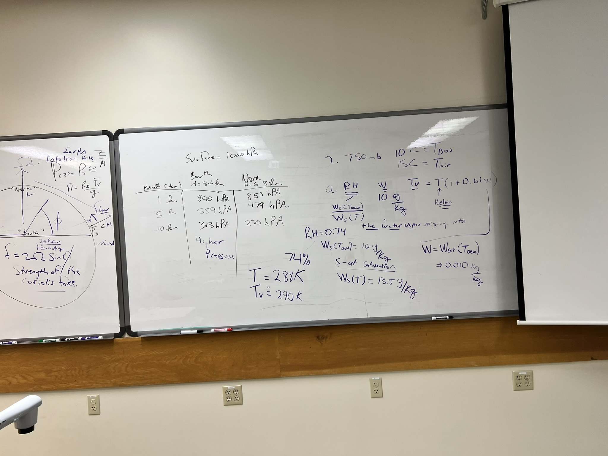
1. Air in the north has an approximate scale height of 6.8 km. In the south, it is 8.6 km. Assuming they both have a surface pressure of 1000 hPa, calculate calculate the pressure at 1 km, 5 km, and 10 km. Based on this, what direction would wind go, toward the north, south, east or west at 10 km?
Answer:
| Height (km) | Pressure, south where H=8.6 km (mb) | Pressure, north where H=6.8 km (mb) | Pressure Difference (mb) |
| 1 | 890 | 863 | 27 |
| 5 | 559 | 479 | 80 |
| 10 | 313 | 230 |
83 |
Wind expected first from the south and then from the west in time as the Coriolis force affects the motion.
2. An air parcel at 750 mb has a dewpoint of 10 C and an air temperature of 15 C.
a.
Find its relative humidity, water vapor mixing ratio, and virtual temperature in Kelvin.
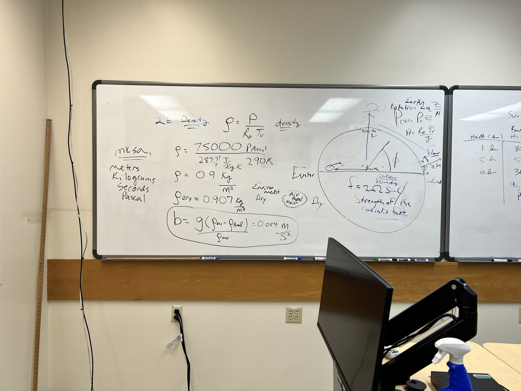
b. Calculate its density if it were dry (dew point 0 K) and at its RH.
c. Assuming that the moist air is an air parcel in in its dry environment, calculate its buoyancy, b=g(ρenv - ρparcel)/ρenv.
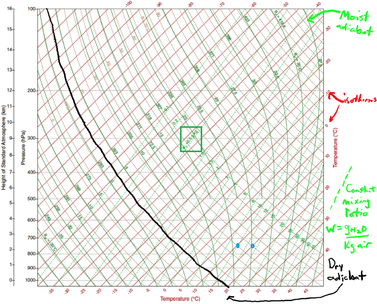
Answer: SkewT diagram. a. RH=wsat(Tdew) / wsat(T) = 10 g/kg / 13.5 g/kg = 74%. w=wsat(Tdew) = 10 g/kg T=288 K. Tv = T (1 + 0.61w) = 290 K b and c. ρ = P/RDTv RD=287.1 J/kgK ρdry=0.907 kg/m3 ρ=0.900 kg/m3 b=0.054 m/s2 |
Board 1, board 2, fire 1, fire 2, fire 3.
Monday - Tuesday
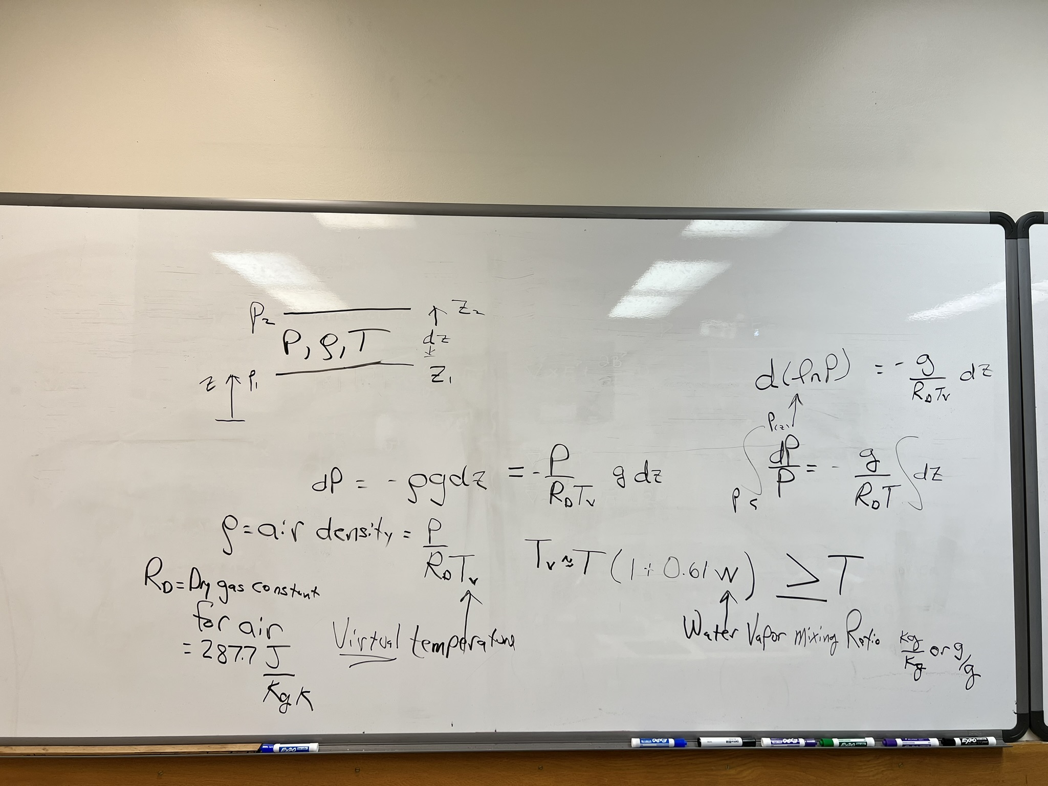
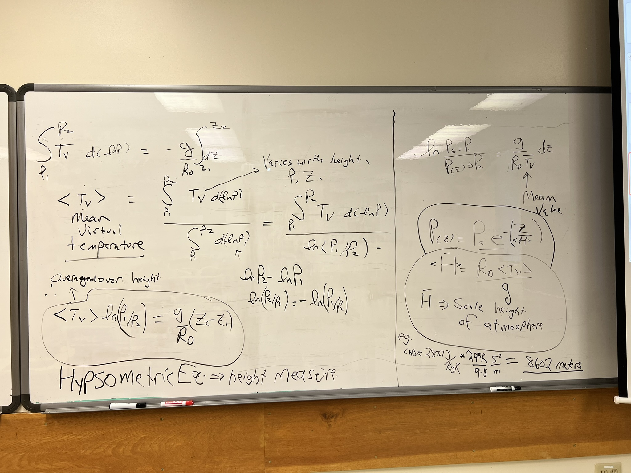
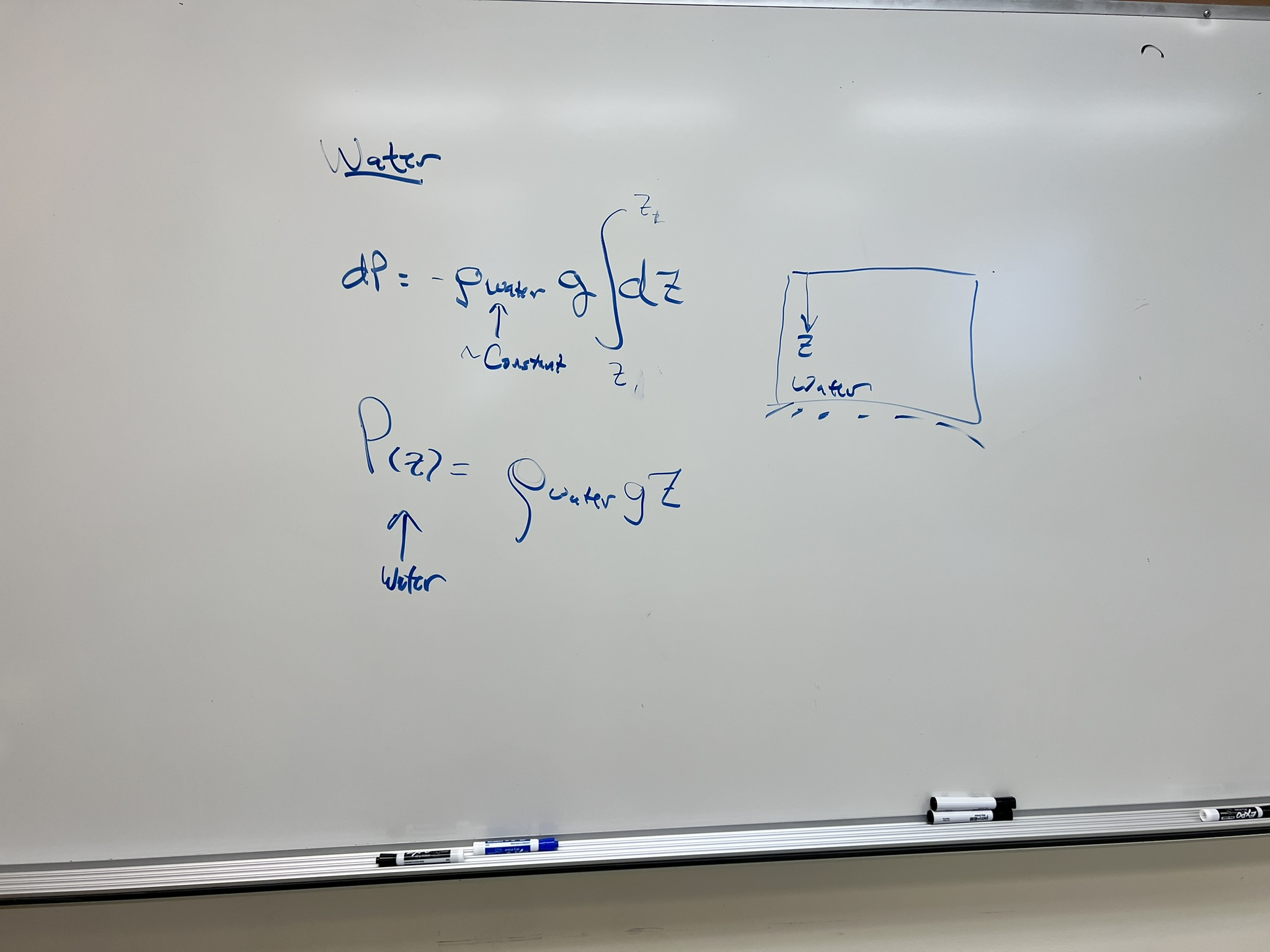
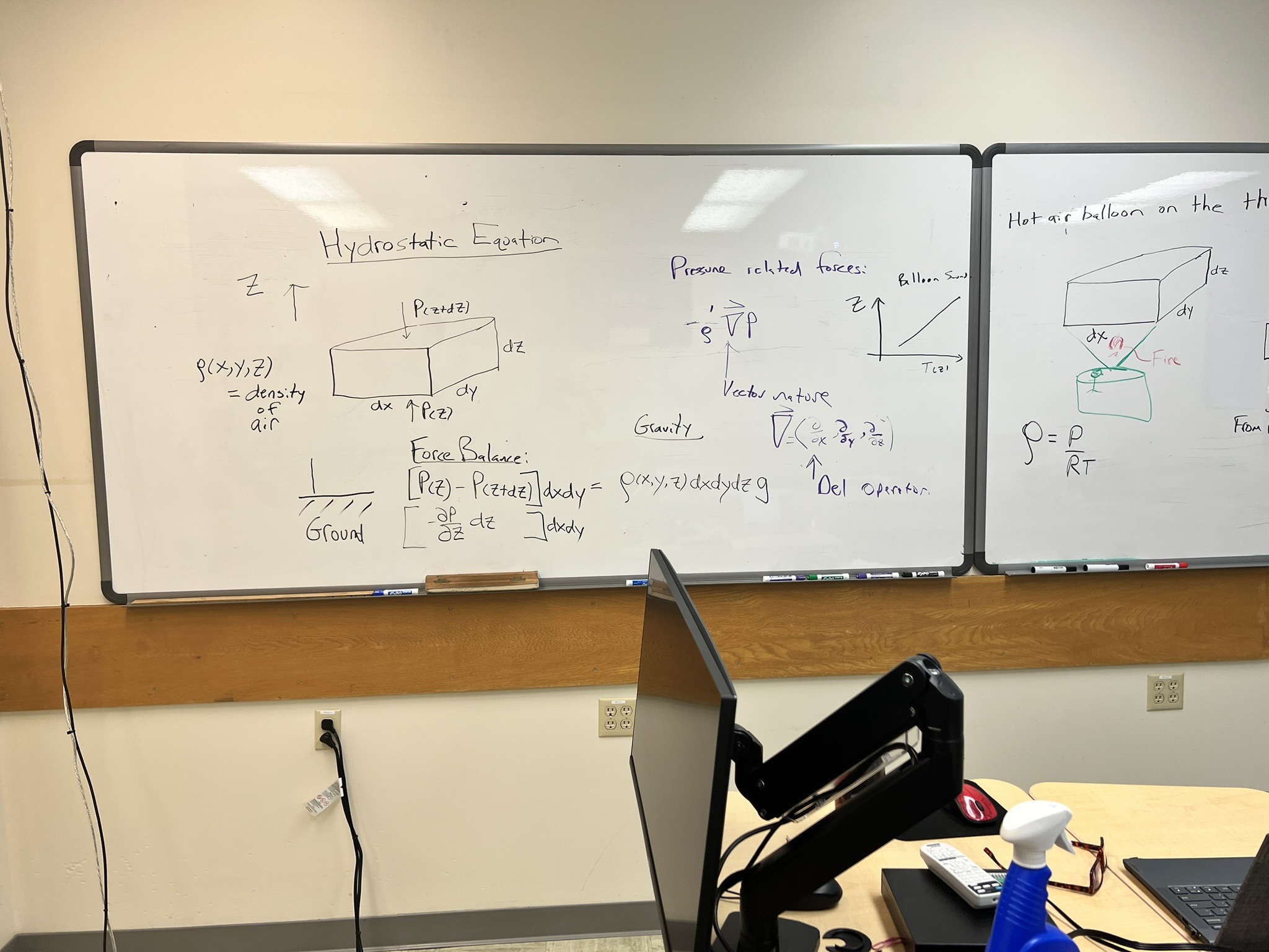
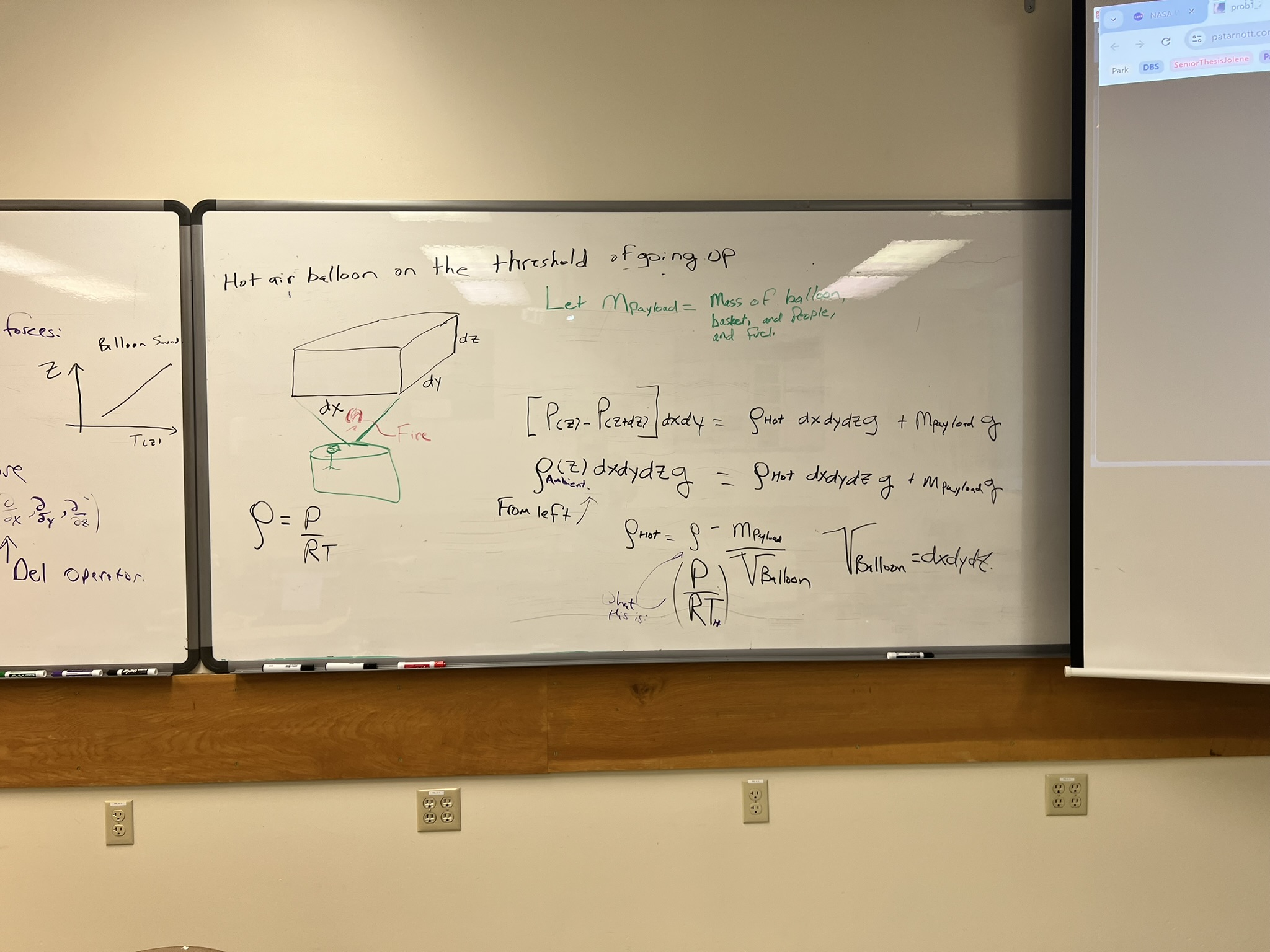
Hydrostatic equation, virtual temperature for use to obtain the correct density, exponentially decaying dependence of pressure with height, pressure in water. Pg1, Pg2, and Pg3.
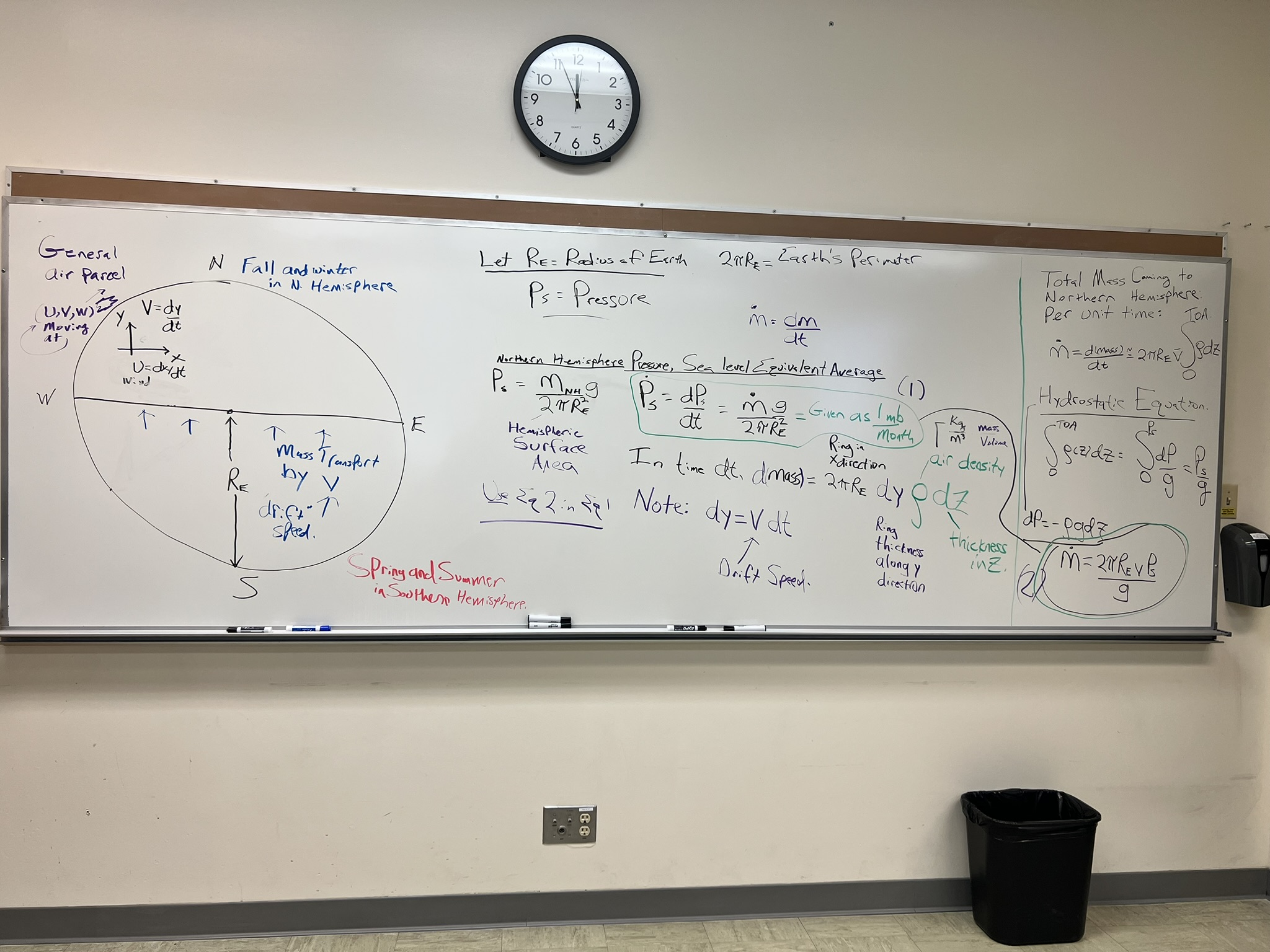
Problem 1.21 analysis and discuss the averaged hemispherical pressure from the homework page.
Whiteboard notes pg1, pg2, and pg3.
Discuss Homework 3. Everyone choose a sounding from a different month.
Install the Anaconda/Python interpreter for the HW3 script.
To create a recent model sounding using HRRR, start at the Continental US scale and click on any point. This will bring up a sounding. Choose on where radar indicates active precipitation, and compare with another elsewhere. Notice the Dendrite Grow Zone (DGR) elevations and associated temperatures.
Week 3: 8 Sept
Thursday
Talk about HW2 South Pole lapse rate and sea level equivalent pressure changes in summer and winter.
Fire field project description (Eliza).
Problem 1.21 analysis and discuss the averaged hemispherical pressure from the homework page.
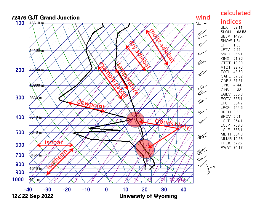
Grand Junction Colorado example of a lifted air parcel from the averaged 50 mb from the surface mixing ratio and potential temperature (image). Excel analysis to get lifted air parcel starting point for LCL and CAPE.
Surface layer, near-surface friction to air motion over water and land, dependence on turbulent boundary layer, and finally, above, geostrophic flow is possible.
Tuesday and Wednesday
Presentations continue for HW1.
Week 2: 31 August
Thursday
Start presentations for HW1.
Tuesday and Wednesday
Discuss the free atmosphere and planetary boundary layer from the Monday soundings. Work towards HW 2.
Monday
Discuss dry adiabats: from PVγ = constant for a gas at pressure P and Volume undergoing an adiabatic process to potential temperature. Dry adiabats on the SkewT diagram.
Reno sounding from yesterday afternoon and this morning.
Bring questions to class on HW 1.
How to read skewT ln P diagrams. (local backup).
Overview Presentation: Work towards HW 2.
Stationary lee wave clouds downwind of the Sierra Nevada mountains.
Week 1: 24 August
Tuesday - Thursday
Work on HW 1.
Overview Presentation: Note the large hail in South Dakota, and thus the need to work on hail suppression.
Stationary lee wave clouds downwind of the Sierra Nevada mountains.
How to read skewT ln P diagrams. (local backup).
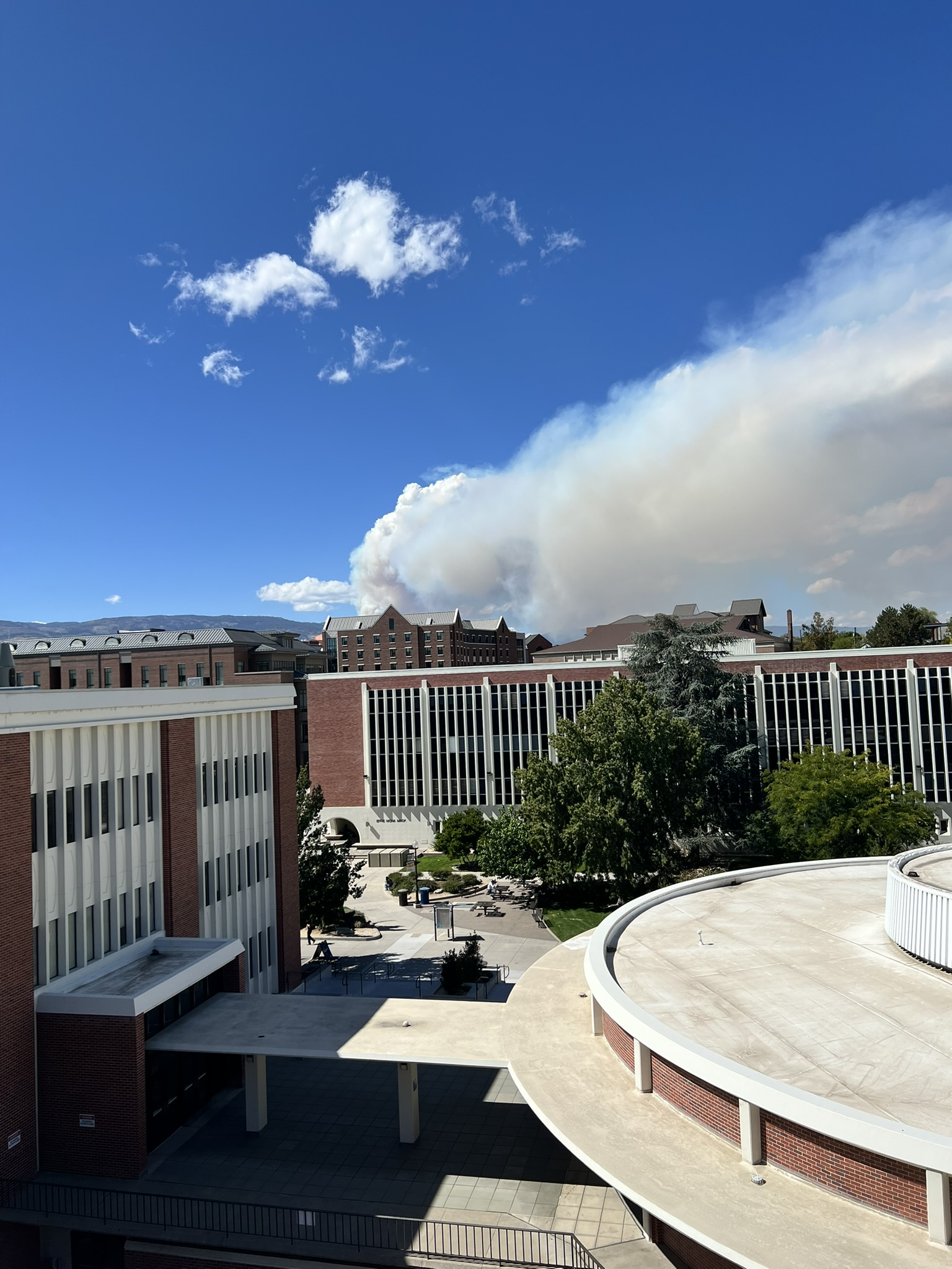
Do a Convective Condensation Level example for how much heating the atmosphere must have to get a pyrocumulus cloud associated with wild fires (CCL).
MODIS imagery from August 19th 2020 (fire detection and vast amounts of smoke).
NOTE: SkewT ln P images can be obtained from:
|
Monday
Outcome: Student introductions, syllabus, homework discussion, and started discussion of Atmospheric Physics, especially fires, smoke and clouds.
Thanks for the questions 😀 I appreciate them immensely!
| Introductions -- each student introduce themselves. |
| Syllabus. |
| Homework. |
| Webcampus for online homework assignments/reading. |
|
Online Homework 1 is due August 30th. See webcampus. Online Homework 2 is due September 6th. See webcampus. Homework 1 is due September 4th, to be turned in through web campus. For this week: Read chapter 1, introduction to large scale features of the atmosphere. |
The final project has been posted. |
This class includes:
Lecture/discussion in class.
Active class participation/activity involving atmospheric data from around the world.
Study using online modules for atmospheric science education.
Chapter 1: Introduction and overview:
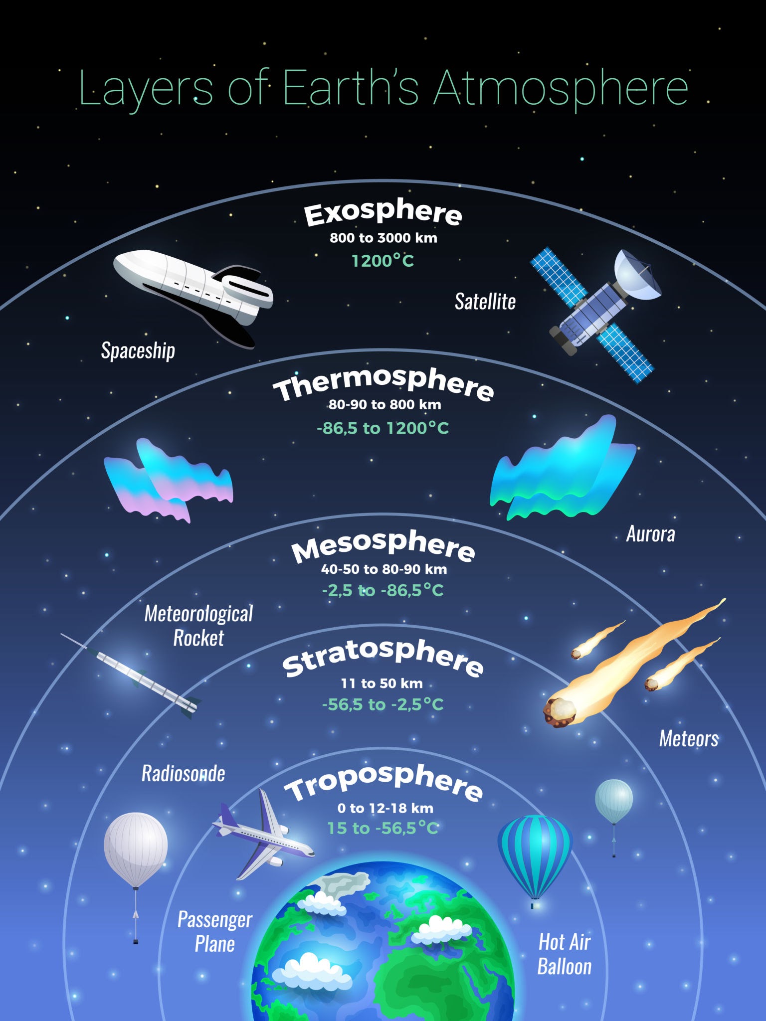
The layers of the Earth's atmosphere.
Vertical structure of the atmosphere.
Overview Presentation: Atmospheric Science relies heavily on measurements and models!
Composition of the Earth's atmosphere.
Related Information: