ATMS 401 Homework [Main Page] [HW4] [Daily Notes] [Final Project]
ONLINE ASSIGNMENTS AND DUE DATES FOR THEM ARE GIVEN IN WEBCAMPUS.
Eliza, Loyalton Fire, August 14-26, 2020.
Sean, Houston Derecho, May 16, 2024 between 6 and 7 pm LDT.
Ricky, February 26th, Oklahoma and West Texas severe weather outbreak.
Graham, September 18th, 2026, Fruit Heights UT Tornado.
Felicia, July 8th 2020, EF4 tornado, in Minnesota.
Farhana, EF4, Marietta, Georgia.
Steps A-G guide you through acquiring your data and intrepreting it,
followed by presentation instructions.
A. Find an exciting sounding (using the Univ. of Wyoming site) (Analysis can be accomplished with this python script) from anywhere in the continental US, after February 28th, 2017, with a lot of convective available potential energy (CAPE).
The limitation on date comes from the availabilty of satellite imagery.
Fire related pyrocumulonimbus/firenados are also encouraged for students working on wildland fires. They are a form of severe storm for the Western US.
Find a nearby sounding and/or generate a model sounding from this HRRR model script.
Find a sounding that was associated with severe weather in the vicinity.
Use archived radar data, or this if the first link doesn't work, for obtaining a quick look at precipitation in the vicinity, time and location of your sounding.
Use also NASA AQUA MODIS for around 2 pm local time quick-look at the area. The city name and state can be used in the NASA Worldview search bar.
Obtain and save both the GIF skew T image and the text file.
The text file will be used for analyzing the sounding, for graphs and for reading values from it.
Color your sounding using the Paint program (or other) to illustrate the level of free convection, equilibrium level, LCL,
and regions of positive and negative buoyancy (green for positive, red for negative).
Here's an example.
Check your sounding for issues like these.
I will be using the Reno 3 July2021 0Z
sounding for the in-class example, so this one is not available for use. Local backup.
Text for the sounding. Local backup.
B. Identify the level of free convection and the equilibrium level.
These can be read from the sounding indices, or at the intersections given by the lifted surface parcel and environmental air.
C. Note and discuss the CAPE, CIN, and precipitable water from your sounding.
Calculate and report the maximum vertical updraft speed in m/s and mph.
wEL=(2CAPE)1/2. Here EL is the equilibrium level.
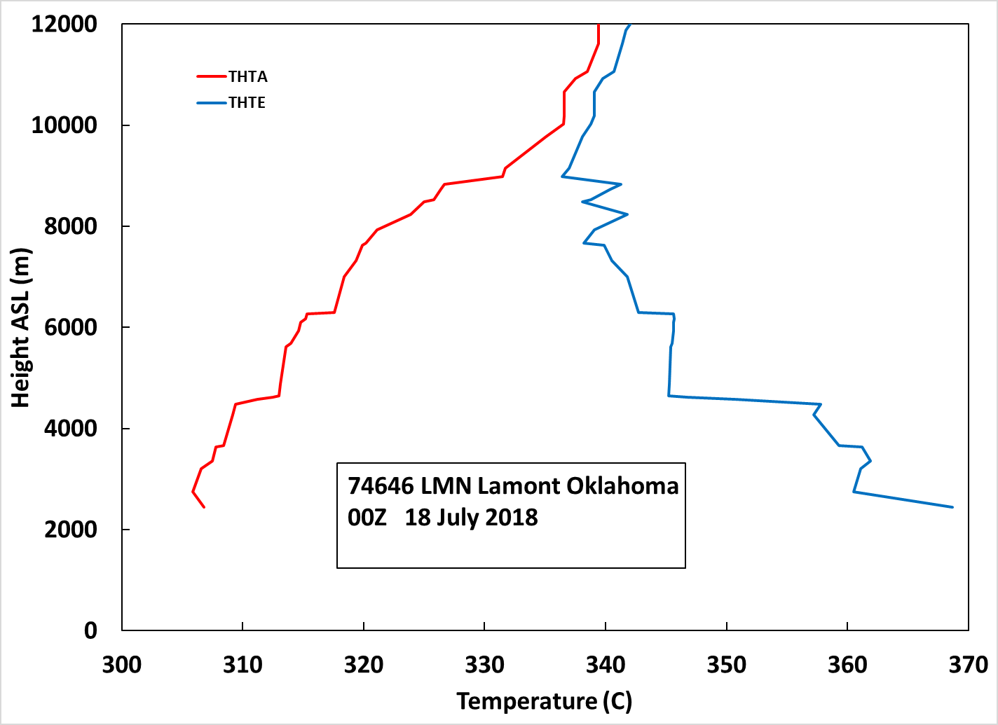
D. Make a graph of the vertical distribution of potential temperature (THTA in the sounding text) and equivalent potential temperature (THTE in the sounding text).
In your discussion, identify stable, unstable, neutrally stable, and convectively unstable regions.
Here's an example; the top height is at just above the equilibrium level.
Plotting these to just above the equilibrium level (and not the top of the sounding) allows us to see the details in the troposphere.
E. 500 mb wind from reanalysis and comparison with your sounding.
It will be helpful to visualize the wind to use the Earth Winds viewer to see the atmospheric circulation at 500 mb near your location. Click on the Earth icon on the bottom left; choose the 500 mb level, and the date of your event. Then zoom in on your location, leaving room to see what's going on near it. Click on where you think the location is, and notice the latitude and longitude of that point. Click until you get the green circle to be centered close to the latitude and longitude given for your location on the sounding in the top right corner. CAPE can be overlain with the image.
Obtain the 500 mb height map from reanalysis for your sounding for the time of the sounding, and including the location of your sounding.
Here is the link for reanalysis data. Settings example.
The latitude and longitude range for your graph can be centered at the balloon observation by finding the latitude and longtitude for it, and going +-20 degrees north and south, and west and east for the bounding box.
Interpret in terms of locations of low and high heights, and wind speed maxima and minima.
Compare the 500 mb wind speed and direction at your location (that should be the map center) with the sounding value at 500 mb.
Here's an example from the 28July2017 0z, Lamont Oklahoma located at about 36.62 North and 97.48 West: Settings and 500 mb plot example. Lamont Oklahoma is in the center of the image.
Lamont OK is site location 74646.
Draw an arrow showing the 500 mb wind direction at your site (center of the graph) based on the height contour spacings and compare with your sounding wind speed and direction at 500 mb.
F. Obtain the radar data animation for your location and its vicinity, and for the time around your sounding.
Radar quick look data for use in scoping your location:
Use this archived radar data tool, or this if the first link doesn't work, and obtain data in and around the time of your sounding, as a screen shot if needed.
Making the radar data animation:
Here's where you choose the radar using COD Radar. Click on "Radar Selection" and it will bring up a map of the NEXRAD sights in continental US.
Find the one closest to your sounding location (or weather event) and hover over it to get the abbreviated name and location that will be needed in the Weather and Climate Toolbox.
Find the coordinates of your radar for locations in the continental US (for Alaska, Hawaii, etc you'll need to estimate the coordinates).
Detailed instructions for obtaining radar data.
Obtain the Level II (choose radar elevation that works best using 'Properties') from the NOAA Weather and Climate Toolkit described in G, to make a movie of the radar data.
Additional Information on Radar:
Excellent Radar Education. Radar presentation. Nexrad radar discussion, and what's under the dome video.
Examples:
Here are a 3 hour animation, and a 24 hr animation obtained for the Reno 3 July 2021 0z case study, showing an outflow boundary, from the lowest elevation scan.
Most of the white color is noise in these animations. The precipitation scales from green to red (20-55 dBz).
G. Geostationary Operational Environmental Satellite (GOES) Infrared Imagery Single Picture and Animation:
Interpretation of satellite infrared imagery of the atmosphere and surface.
First, use the NOAA Weather and Climate Toolkit (WCT) to get an infrared image for the time of your sounding to use in identifying cold cloud tops (low radiance values) associated with convection.
We will use GOES 16 or GOES 19 (after 2023) data for coverage of the entire continental U.S.
NOTE: We willl change the color table Rainbow 3, and flip so that red warm colors correspond with the lowest radiation amount and cold cloud tops high in the atmosphere.
Detailed instructions for obtaining GOES data.
Here's an example of a query. And here is an example image.
The data is "Clean" Infrared Longwave Window Band. The center wavelength for this band is 10.3 microns, or a wavenumber=970.9 cm-1. (wavenumber=1/wavelength).
Estimate cloud top temperature for convection in the area assuming cloud top is a blackbody radiator.
You can hover over locations of interest when in WCT and read the infrared radiance.
Then use the measured cloud top radiance in this calculator to get the brightness temperature.
Second, create an GIF or mp4 animation of the location for several hours around the time of the sounding. Tutorial on making animations.
Presentation Suggestions:
Introduction:
Discuss CAPE and precipitable water vapor amount in the introduction.
Be sure to define each variable when using equations.
Section 1. Use Google Earth and the latitude and longitude coordinates of your sounding to create a map of the location in wide enough of an area to give an idea of its climatological context.
You may find useful climate information on your site here. Describe what motivated you to choose your site.
Section 2. Present your skewT graph and its interpretation, including discussion of the wind speed and direction as a function of height; temperature, and dewpoint temperature; and the lifted air parcel. (See step A).
Section 3. Give a table of values for your location and include:
| Quantity | Units | Comment | How to get it from the skewT diagram. |
| CCL Pressure | mb |
Pressure at the convective condensation level (CCL) | The CCL is the level at which condensation will occur if sufficient afternoon heating causes rising parcels of air to reach saturation. The CCL is greater than or equal in height (lower or equal pressure level) than the LCL. The CCL is found by following the saturation mixing ratio line through the surface dewpoint up until it intersects the environmental temperature curve. Adapted from here. |
| Convective Temperature |
C | Surface temperature the air needs to reach to form clouds by thermal convection caused solely by surface heating | Follow the dry abiabat from the CCL back to the surface pressure level. Read the temperature. Note: This temperature is especially useful for studying pyrocumulonimbus formation associated with forest fires. |
Section 4. Graph with all the potential temperature and equivalent potential temperature curves versus height.
Discuss atmospheric stability using these graphs. (See step D).
Section 5. Prepare a 500 mb level graph and discuss it. (See step E).
Section 6. Obtain the radar still image and animation for your location and surrounding area, and discuss them. (See step F).
Section 7. Obtain the infrared satellite still image and animation for your location and surrounding area, and discuss them. (See step G).
Conclusion: Summarize your findings.
Appendix:
a.
You may include any related atmospheric data (like maps of other pressure levels, etc) that helps tell your story.
Resources and Explanations for the NOAA ToolKit
Change the theme in the upper right corner to get something more useful, like streets.
Level 1 data for channel 13: ABI-L2-CTPF is the infrared radiance arriving at the satellite.
Resources for GOES Satellite Imagery on GOES (Geostationary Operational Environmental Satellites):
Overview of how it works. Shorter version.
More details on the satellite instruments.
GOES west real time IR imagery at 10.35 um, converted to brightness temperature. Close look at California and Nevada. Imagery from GOES east.
LEVEL 2 PRODUCTS
Definition of the level 2 derived data types in the toolkit.
ABI-L2-CTPF is the cloud top pressure.
ABI-L2-ACHAF if the cloud top height.
ABI-L2-ACHTF is the cloud top temperature.
Tools and Extras
0. Soundings from the University of Wyoming site. Python script for this assignment.
1. Experimental HRRR model sounding Python script.
2. You may also obtain archived data for the 500 mb level, and precipitation data from radar imagery here.
3. Historical weather may be obtained here, mostly from surface stations at airports.
4. Historical surface analysis showing highs and lows and fronts are available (scroll down).
5. Archived satellite imagery from around the world can be obtained here.
6.
Read section 8.3.1a on Deep Convection, pg 344-371 of Wallace and Hobbs for getting a better understanding of severe storms.
7. Skew T plots discussion.
8. Archived weather radar.
9 Severe storms 101 discussion from the National Severe Storms Lab.
10 Newscast discussing severe storms and tornados.
11. Ingredients for a thunderstorm and severe weather.
12. Radar Doppler discussion.
13. Radar reflectivity and interpretation.
14. Thunderstorms.
15. The 500 mb pressure chart.
16. Satellite imagery interpretation in brief.
17. Tornado formation discussion.
18. Example analysis of Enderlin, 21 June 2025 EF5 tornado. (Don't use this case).
19. This assignment primarily concentrates on CAPE.
Dynamical meteorology has a strong effect on severe storm outcomes.
Further discussions are in the MetEd modules on Principles of Convection 2: Using Hodographs and Principles of Convection 3: Shear and Convective Storms.
|
|
Journal Articles
Soundings associated with supercell storms.
Effect of entrainment on CAPE.
Evolution of Convective Energy and Inhibition before Instances of Large CAPE 2023. (Backtrajectory analysis used to look at origin of air masses).
Additional, Optional Severe Weather Software: Python program and executables for viewing observed and modeled soundings in the context of severe weather description.
OPTIONAL: Using the sounding text, calculate the CAPE in units of Joules/kg, the estimated vertical velocity at the equilibrium level in meters/second and compare with the value on the sounding.
Also, calculate the precipitable water vapor amount in units of mm and compare with the values given on the sounding.
This spreadsheet will help you calculate temperature along the moist adiabat and gives an example for CAPE and precipitable water calculation.
Replace the example sounding with your own and redo the calculations.
(Here's another version; it also has the calculation of the moist adiabatic lapse rate.) I can assist if you would like to work with the program.
You can also make your own program with any language you would like to do this calculation.
Explain what program you use, and include it in the report.
Make one document that has solutions for problems 1 through 4.
Read chapter 3 and .
Read about them from various sources and then from understanding, discuss them.
Describe how to obtain them using a skew-T diagram or from calculation.
a. Tv virtual temperature
b. Tdew dew point temperature
c. Tw wet bulb temperature
d. Tc convective temperature
e. θ potential temperature
f. θw wetbulb potential temperature
g. θE equivalent potential temperature
a. Dewpoint temperature from the temperature, pressure, and wetbulb temperature.
b. Wetbulb temperature from the temperature, pressure, and dewpoint temperature.
Ambient temperature To=25.7 C, wet bulb temperature Tw=14.1 C and ambient pressure Po=865 mb. (Obtained on 10/1/2026 outside).
Deliverables for problem 3:
Some of the calculations needed for the table below can be checked using the National Weather Service water vapor calculator.
| Quantity | Units | Value from skewT | Comment | Procedure using skewT |
| Tdew | C | dewpoint temperature | Use Normand's rule | |
| ws(Tdew) | g/kg | water vapor mixing ratio at saturation at the dewpoint temperature | Read from the skewT | |
| ws(Tw) | g/kg | water vapor mixing ratio at saturation at the wetbulb temperature | Read from the skewT | |
| ws(T) | g/kg | water vapor mixing ratio at saturation at the air temperature | Read from the skewT | |
| RH | % | Relative humidity | RH=ws(Tdew)/ws(T) | |
| θ | K | Potential Temperature | Follow the dry adiabat through T down to P=1000 mb and read the temperature. | |
| θw | K | Wetbulb Potential Temperature | Follow the moist adiabat throughTw down to 1000 mb and read the temperature. It can also be read in the upper level of the skewT we use for class. | |
| θE | K | Equivalent Potential Temperature | Use Normand's rule to get to the LCL. Then follow the moist adiabat to the top of the atmosphere. Return to 1000 mb along a dry adiabat and read the temperature. It can also be read in the upper level of the skewT we use for class. | |
| LCL Temperature | C | Temperature at the lifting condensation level (LCL) | Use Normand's rule | |
| LCL Pressure | mb | Pressure at the LCL | Use Normand's rule |
At the center of a hurricane is a warm core low pressure region, the eye of the hurricane.
This table gives a categorization of hurricanes by maximum wind speed range. (local backup).
a. Discuss the life cycle of hurricanes: formation, energy source, and dissipation (be sure to cite your references, see Resources. This is not just a bibliography.)
Discuss especially why the eye of the hurricane is mostly clear of clouds, and why the surface wind in the eye wall is so strong.
How do hurricanes separate the updraft and downdraft?
b. Create a 'hurricane' table with headings Category, Sustained Wind Range (m/s), Eye Pressure Range (mb), Average Eye Temperature Difference (C).
We will use cyclostrophic flow theory in class to show that the pressure difference between the eye and the surroundings is ΔP=1.81ρv2 where ρ is surface density and v is maximum hurricane wind speed. The pressure at the eye of the hurricane is Peye=Po- ΔP. Be sure to convert the units of ΔP to mb.
Use the eye and surrounding pressure to assumed to be 1010 mb to obtain the average temperature difference between the atmospheric column above the eye and surroundings (see prob 3.26).
[We showed that ΔT=Toln(Po/Peye)/ln(Peye/200mb) where To=-3 C = 270 K, and Po=1010 mb.]
Here's an example of the table for the first entry. It's convenient to use Excel for the table.
Section 8.4 pgs 366-371 of the class textbook, .
Hurricane Freddy, Southern Hemisphere 2023, longest lived and most energetic in history.
NOAA's hurricane division and description of hurricanes.
This paper discusses hurricane properties.
This paper discusses the dynamics of a specific hurricane in detail, including the effect of temperature on hurricane strength.
Additional papers:
Extreme low-level updrafts and wind speeds measured by dropsones in Tropical Cyclones 2016.
Electrification of hurricanes 1998.
Extra large particle images at 12 km in a hurricane eyewall: Evidence of high-altitude super cooled water? 2003
You can reference it in your report, comparing your values with those in the paper, and find other references for hurricanes using the Web of Science.
We will discuss in class how to use cloud applications for EndNote and WebOfScience to manage references within Microsoft Word (download and install the Endnote plugin for Word).
We did problem 3.26 in class to develop theory for the average column temperature difference and the hurricane eye pressure given the wind speed.
National Hurricane Center site and data.
Numerous websites talk about the circulation in hurricanes.
Hurricane Ian discussion on Tuesday, on Wednesday and on Thursday, September 27-29, 2022.
The powerpoint presentation for chapter 3 may be useful. The hurricane problem is there.
Homework 3
Title: Case study of a polar and tropical meteorology: Radiosonde analysis.
Reading: Chapters 1 and 3 and provided links.Turn in through WebCampus, prepared using Microsoft Powerpoint, and present.
CASES: (Hint, try to pick a day and time in a month not represented already).
JP: 30 July 2020 0z
FL: March
SB: August 16, 2025, 0Z
EF: February 21, 2026 12Z
GW: November 25, 2020, 0Z
MG: August 25, 2020, 0Z
RC: May 26, 2022, 0Z
EH: June 20, 2026 12Z
LM: July 11, 2026 12Z
AC: August 12, 2026 12Z
FM: January 16, 2026 0Z
JP: July 7, 2023, 0Z
Purpose
- Access and interpret sounding and reanalysis meteorological data from around the world.
- Calculate and graph meteorological variables to investigate their vertical distribution in the atmosphere.
- Learn to make and interpret publication-quality meteorology graphs.
- Advance science presentation skills.
- Calculate integrated vapor transport (IVT) for quantifying Atmospheric Rivers (more info). More sophisticated version.
- Atmospheric river discussion.
- Use a solar radiation simulation application for any time and location.
Instructions
We will go through this problem together in class.
Ask questions.Here is a Python script to use for most of the graphs needed.
The program 'Spyder' within Anaconda can be used to run this script, for example. (Installer).Google Colab can be used as well.
Prepare by getting a Google account if you don't have one.
Actions within Colab:
1. Create a new folder.
2. ! wget https://www.patarnott.com/atms401/HW3_Roch_Barrow2026.py (USE SHIFT ENTER TO EXECUTE THIS AND LINES BELOW.)
3. ! pip install metpy
4. ! pip install siphon
5. ! python HW3_Roch_Barrow2026.py
Colab gives us full access to a Bash shell (among other things).
Prepare a presentation that describes the atmosphere for these two locations, Rochambeau French Guiana (SOCA, Station 81405) and Barrow Alaska USA (PABR, Station 70026) for the date and time of your choice.
Send me the date and time of your study (arnottw at unr dot edu) and I'll post it here to make sure we don't have overlap with others.
Use the high spatial resolution sounding data and make your presentation from the Assignment Tasks below.
Assignment Steps
a. Locations: Use Google Earth to view these two locations, Rochambeau French Guiana (coordinates 4.8222, -52.3653) and Barrow Alaska USA (coordinates 71.2889, -156.7833).
Save images of each location and use as figures 1 and 2 in your presentation.
Include grid lines (turn on with the menu item View:Gridlines) in these images and adjust the magnification so that you can see the Equator and the Tropic of Cancer, and for Barrow the Arctic Circle. Briefly discuss the significance of the Tropic of Cancer and the Arctic circle in general and with respect Rochambeau and Barrow, and qualitatively, the amount of solar radiation they receive seasonally.
b. Skew-T Diagrams: Acquire the png format skew T soundings from the Wyoming site, or use the Python script, for PABR and SOCA for this day and time. Make these soundings figures 3 and 4 in your presentation.
Discuss these soundings. What is the local standard time at each site for the soundings?
Discuss the lapse rate Γ=-dT/dz from the slope of the temperature versus height graph at any point and interpret, along with other feature observed.c. Rochambeau Data: Near equator: Rochambeau French Guiana (get sounding text for SOCA from the Wyoming site, or use the Python script.)
Plot pressure and temperature vs height in km as figure 5 in your presentration, with pressure on the lower x axis, and temperature on the upper one.
Calculate density and plot versus height in km as a separate graph as figure 6.
Density of dry and moist air d. Barrow Alaska Data: Near north pole: Barrow Alaska (PABR).
Get the text sounding data for PABR from the Wyoming site, or use the Python script.
Overlay pressure and temperature vs height in km with the SOCA pressure and temperature in figure 5.
Calculate density and overlay with the SOCA density in figure 6.
Additional problem for ATMS 601 student and extra credit for ATMS 401 students:
- Interpolate the pressure measurements from SOCA and PABR to a common height grid and calculate the 5 times the pressure difference = 5*(PABR - SOCA) as a function of height. The height grid starts at 22 meters and ends at 25927 meters and goes in steps of 11 meters. Here's an example of previous interpolated data obtained from this python script. The pressure difference values should be negative when aloft, or use the Python script.
- Add this calculation to your presentation.
- Discuss the following questions.
- How does the maximum in the magnitude |PABR-SOCA| relate to the PABR temperature profile?
- What is the dynamical significance of the maximum with regard to large scale circulation in the atmosphere? Estimate the geostrophic wind speed for the maximum pressure difference. Here are notes on wind speed estimation (PDF format) and (OneNotes , right click and save to a file. Open with OneNote.)
- What might be the consequence of rapid warming in the Arctic on the large scale circulation?
e. Water vapor density: Calculate and graph the water vapor density in grams/m3 for Barrow and overlay with the SOCA water vapor density, as an overlay with figure 6.
Note that water vapor density is the product of density_of_dry_air * w. Discuss.
f. Atmospheric river (AR) related analysis. Transport of water vapor.
Note: To understand the total mass transported by an atmospheric river requires more than 1 isolated balloon sounding. This problem is to aid in understanding the primary quantity needed for the first step, quantifying the transport of water vapor by the wind in a column of the atmosphere.
Calculate the vector Integrated Vapor Transport (IVT) (units of Kg/(m s)) and total precipitable water vapor (PWV) (units of mm) for both Barrow and SOCA.Here is a summary of the relationships needed, repeated in this table.
Summary of relationships for water vapor transport description.
Click on images for larger versions.
The average velocity vector for water vapor transport is equal to the IVT/IWV, where IWV=total integrated water vapor.The purpose is to become familiar with this important concept used to described Atmospheric Rivers.
Here are some notes in OneNote format, and in PDF format.
This research paper describes IVT in Eqs. (1) - (5).
This site describes wind as a vector and its speed and direction.
This site describes operational forecast for atmospheric rivers, and water vapor transport analysis.
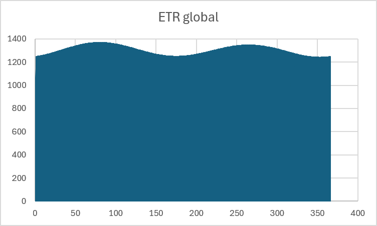
g. Solar Radiation: Use this solar position and irradiance calculator (from the National Renewable Energy Lab) to simulate the top of the atmosphere solar irradiance for a detector placed flat on the ground (horizontal detector) every 30 minutes for Jan1 - Dec31, for SOCA and PABR.
It also known as the "Extraterrestrial Global Horizontal Solar Irradiance (W/m2)". We will use the acronym EGHSI for it.
The results will be a time series of top of atmosphere irradiance values that need to be brought into Excel and plotted. The x-axis will be the day of the year calculated by first combining time and date into a new column, and then using the equation given here.
Make these figures 7a and 7b, on one page for ease of comparison. Discuss these figures in the presentation.
This image shows the setup for getting numbers for SOCA (change latitude and longitude to get PABR numbers), and this image show which field to use for the irradiance (the temperature and pressure don't matter in the first part).
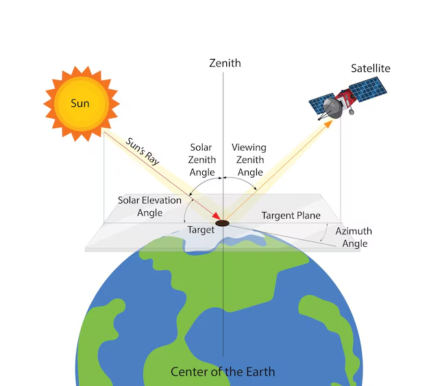
The Earth's orbital path around the sun is elliptical rather than circular. Note that the solar zenith angle, which is the complement of the solar elevation angle, affects EGHSI more than variation of the Earth-Sun distance as discussed here. This simulation is useful for understanding the Earth's tilt and its effects on seasons, in addition to the variation of irradiance due to the Earth-sun distance. Zooming in the SOCA data to an irradiance range from 1200 to 1400 Watts/m2 shows both the effect of solar zenith angle and the asymmetry for the yearly maximum due to the time of the peak and minimum Earth-sun distance as compared with the time of the solstices.
After getting data on the webpage, do the following within Excel (or other programs) to make a graph:
ctrl a. (select all)
ctrl c. (copy to clipboard).
new excel workbook.
click on cell A1.
ctrl v. (paste)
click on the entire A column by clicking on the A.
click on menu item Data:Text to Columns: Delimited: Commas (delimeter)
Right click on A and insert new column
Enter the formula = B2+C2 into A2 and spread it down by double clicking on the little square in the bottom right of A2.
Right click on A and insert a new column.
click on A2 and enter =B2-DATE(YEAR(B2),1,0) to get just the day of year.
Propogate this down by clicking on the little square in the bottom right of A2.
Click on Insert:Charts:Scatter:5th choice. Your graph should look like this. Clean it up for presentation with axes labels, etc.
Example rough graph for SOCA and spreadsheet.
In summary:
Compare and contrast the difference in the meteorology between these two sites as a function of height in the atmosphere, both near the surface and throughout the atmosphere.TOOLS
- Meteorological data can be obtained from the University of Wyoming web site.
- Students can download Microsoft Office for their home computer. Excel and Word are available for students and faculty here. Sign in with your UNR netID and download Office to your computer.
- It is useful to import data using the text wizard: Excel:File:Options, then check this box.
- Description of balloon soundings of the atmosphere.
- References to published papers and websites can be easily managed with EndNote online. Scroll down to "Manage your references" for instructions.
- Optional Python script to plot the balloon trajectories in Google Earth, by creating a .kml file that can be read directly into Google Earth. Get data from the U. Wyo site: use the "Output Data : Comma Separated Values" to get the radiosonde data from the high resolution sounding page.
Homework 2. Chapter 1.
Turn in this homework assignment through webCampus.
Make one document (it can be photographs of hand-written problem solutions placed in MSWord or other programs) with solutions for problems 1 through 3.
- Purpose:
- Study chapter 1 for an overview of Atmospheric Physics.
- To become familiar with the Antartica, South Pole sounding site (station 89009).
- Consequences of gentle air migration from the spring hemisphere to the fall hemisphere.
Read chapter 1.
1. Do problem 1.6 parts a, c, d, and i from the textbook. Write your answers into the first part of the MSword document you will be turning in for this assignment.
2. Do problem 1.12 from the textbook, being sure to express your answer in degree C per kilometer, and be careful with the sign of the value you find.
Go to the Amundsen-Scott station at the South Pole, Antarctica, where radiosonde measurements (station 89009) are sporadically obtained, to see if we can find such an extreme lapse rate as in problem 1.12.
Go to the Univ. of Wyoming radiosonde server, and obtain the South Pole sounding png image and text for 12Z on 28 August 2026. Use the soundng text values to calculate the lapse rate.
Is the surface inversion as small as in problem 1.12? Discuss the South Pole sounding in your report.
3. a. Do problem 1.21 from the textbook. This is similar to problem 1.20 from the textbook we will do in class. Show that the air speed is v=(dp⁄dt) RE ⁄ Ps where RE is Earth's radius and Ps is the average surface pressure. Calculate the air speed and use units of mm/second.
b. Here are graphs of the surface pressure averaged from 1950 - 2019 for Dec/Jan/Feb and for June/July/August.
Discuss the seasonal variation of surface pressure in the Northern hemisphere in summer and winter, locations of highs and lows, and meteorological consequences.
This is discussed an online dynamics textbook near Figure 2.3, the pertinent section is here.
[This data is from NCEP/NCAR. One objective of this problem is to become aware of this data].
[Data from NOAA, Physical Science Laboratory, Monthly/Seasonal Climate Composites]. Historical data is available in another form here.
c. Here is a time series image for this problem, obtained with a web-tool, and this spreadsheet has the details.
Web-based tool for time series development of atmospheric quantities, and intercomparison of reanalysis products.
After looking at the data, is part a. plausible?Resource for problem 1:
Turbulence and vortex rings in air video to visualize the air motions likely happening in the planetary boundary layer and get an introduction to turbulence.Resource for problem 2:
Example Python script that acquires the radiosonde data for June, July, and August, calculates the surface lapse rate, plots it as a time series, and finds the day of the minimum. (Generated with CoPilot AI).Resources for problem 3:
Reanalysis Summary.
Summary of some reanalysis sources.
Site devoted to Meteorological Reanalysis.
Homework 1. Comparison and Contrast of Reno, Nevada, with Slidell, Louisiana.
Turn in this homework assignment through webCampus, using Powerpoint, and present it.Email me (arnottw at unr.edu) your date and time for the sounding so we can attempt to have everyone work on a unique case.
Days and times already taken:
9 Aug 2026 0Z
11 Mar 2026 12Z
24 Nov 2023 0Z
19 June 2026 0Z
24 Aug 2026 12Z
11 Aug 2026 0Z
12 April 2026 12Z
5 Aug 2026 0Z
10 Aug 2026 0Z
23 Aug 2026 0Z
28 Feb 2026 0Z
Skew T lnP Practice. Homework based on the atmosphere and the day and time of your choice in 2026.
We will work on 15 August 2026 at 0Z in class to illustrate the process.
Reno sounding location is 72489 REV (39.56, -119.8). Slidell Louisiana sounding location is 72233 LIX (30.34, -89.83).
Instructions: Place your results from parts 1 through 7 into a Powerpoint Document and submit it to Webcampus. The day for presentations will be announced.
NOTE: SkewT images can be obtained from the University of Wyoming for text values and images;
the College of Dupage for skew T lnP images;
or the National Center for Atmospheric Research (NCAR);
or the Storm Prediction Center (SPC);
or locally (the lifted surface air parcel is included: A screen shot must be used to save data).
Use the blank skewT graph with curves marked, or a blank skewT graph to Microsoft Paint, or your favorite image program.
1. From the Reno sounding text, make a table with the temperature and dewpoint temperature for pressures of mb of 850, 700, 500, 400, and 250 mb. If data is missing at a level, choose the closest value.
2. Put these points on the blank skewT graph using Paint, save your skewT image file.
3. Obtain the sounding as an image, circle the temperature and dewpoint temperature values at the pressures given in part 1.
Compare with your skewT from part 2 with the actual sounding in part 3 to make sure you are understanding these charts.
4. Download the Slidell Louisiana sounding image on the same day and time. Discuss the comparison with the Reno sounding.
5. Make a Google Earth map using the coordinates for each location to help your discussion of the meteorology you would expect for Reno and Slidell.
Google Earth can be downloaded as an application for your device, or used from the web.
6. What are the local daylight savings and local standard times in Reno and Slidell at the time these soundings?7. Obtain the afternoon NASA Worldview (MODIS sensor, Aqua satellite) and use it to help interpret the meteorological differences.
Resources
Some skewT lnP applications and measurements.
Skew T lnP MetEd Module that covers nearly everything, starting with the basics.
How to convert to and from UTC.
Upper air soundings and skewT discussion.
This Python script can be used to plot the balloon trajectories in Google Earth, by creating a .kml file that can be read directly into Google Earth.
Use the "Output Data : Comma Separated Values" to get the data from the high resolution sounding page. Not required but useful.
Time zone in Reno.
World time zone map and Greenwich England.
Current time UTC (Coordinated Universal Time).
World time converter.
Video describing skewT diagrams.
Example of radiosonde errors that can lead to faulty skewT diagrams.
FINAL PROJECT, START SOON!Deliverables:
ATMS 401 in class presentation and turn in presentation in through WebCampus.
ATMS 601 in class presentation, report, and turn in through WebCampus.
Presentations need to be between 15 to 30 minutes long.Take photographs and/or use other data for the atmosphere, and/or investigate a specific topic we haven't covered in class, or covered lightly (such as the ionosphere, or lightning) and explain the Atmospheric Physics connection. The project topic is not limited to obtaining cloud pictures and explaining them, but can be within the rather broad umbrella of Atmospheric Physics. Please check with me if you have questions or want to talk about resources for the project. Project topics can be chosen to support your BS, MS or PhD research topic though should not be on research you have already accomplished prior to this course.
For observational projects, as an example, you can use photographs or data sources, and can look at a variety of phenomena.
For example, blue sky, sky polarization, coronas, halos, rainbows, lenticular clouds, gravity waves, lightning, water phase clouds, ice phase clouds,
inferring air motions and winds from cloud structures, contrails, vortices in contrails, sky color during pollution events, sky color near the horizon, sky color at sunset looking to the east.
Photographs of the dendritic nature of ice growing on windshields on cold days, the shape and nature of icicles, dew on a moist mornings are also possible topics.
Photographs of snow flakes and snow crystals, here's a discussion.
If you have special hobbies or work, like paragliding or mountaineering, Atmospheric Physics related aspects can be included in your project.
You can use soundings, satellite images, weather station data, etc, to also help tell the story.ATMS 401 students will do a presentation. Presentation hints. 7 secrets of great speakers. Teachable moments.
ATMS 601 students will do a presentation and a report. Report format.Grading rubric.
Due Dates:
Before Mid Semester: Submit a tentative title and discussion of the topic you would like to work on for this project through WebCampus.
Presentations: Presentations begin on Wednesday the week before prep day. Prep day is on a Wednesday too. Turn in your presentation through webCampus by Tuesday night.
Reports for 601 students: The Sunday after prep day. They can be submitted as a second file through webCampus.
Resources that may help
Gravity wave discussion.
Snow crystal/flake observations.
Cloud identification.
NASA WorldView for satellite imagery. You can add layers for additional information.
National Weather Service balloon soundings, served by the Univ of Wyoming.
Weather station data from the Western Regional Climate Center at DRI. In particular, the UNR weather station.
Clouds in and near Reno, NV.