Class on Tuesday: 7:30 am to 8:45 am in RM DMS 106 Presentations.
Students will continue to work in groups as described in the Week 12 notes to analyze data and prepare their presentation.
As a group member it's important to do your part, to contribute to the overall success of the group. Each group will have a presentation.
Here's a generic outline for the presentation:
1. Introduction to that part of the campaign you worked on.
Discuss the science associated with your measurements.
2. Show a time series of your data (time on the x axis, and say pressure on the y axis if your group is responsible for the pressure measurements).l
3. Discuss how you did sensor calibration if necessary.
4. Discuss how your sensor works.
5. Intercompare sensor output with time series (for example, data from the UNR station and from the Teensy cards).
6. Discuss and interpret your data (for example, study the time evolution of the pressure and/or temperature for the Teensy card on the balloon sounding system).
7. Wrap up with suggestions for improving the experiment.
Class on Thursday: 8:00 am to 9:15 am in RM DMS 106 presentations as needed to finish up; otherwise radiation measurements to be discussed.
Useful and Related Information:
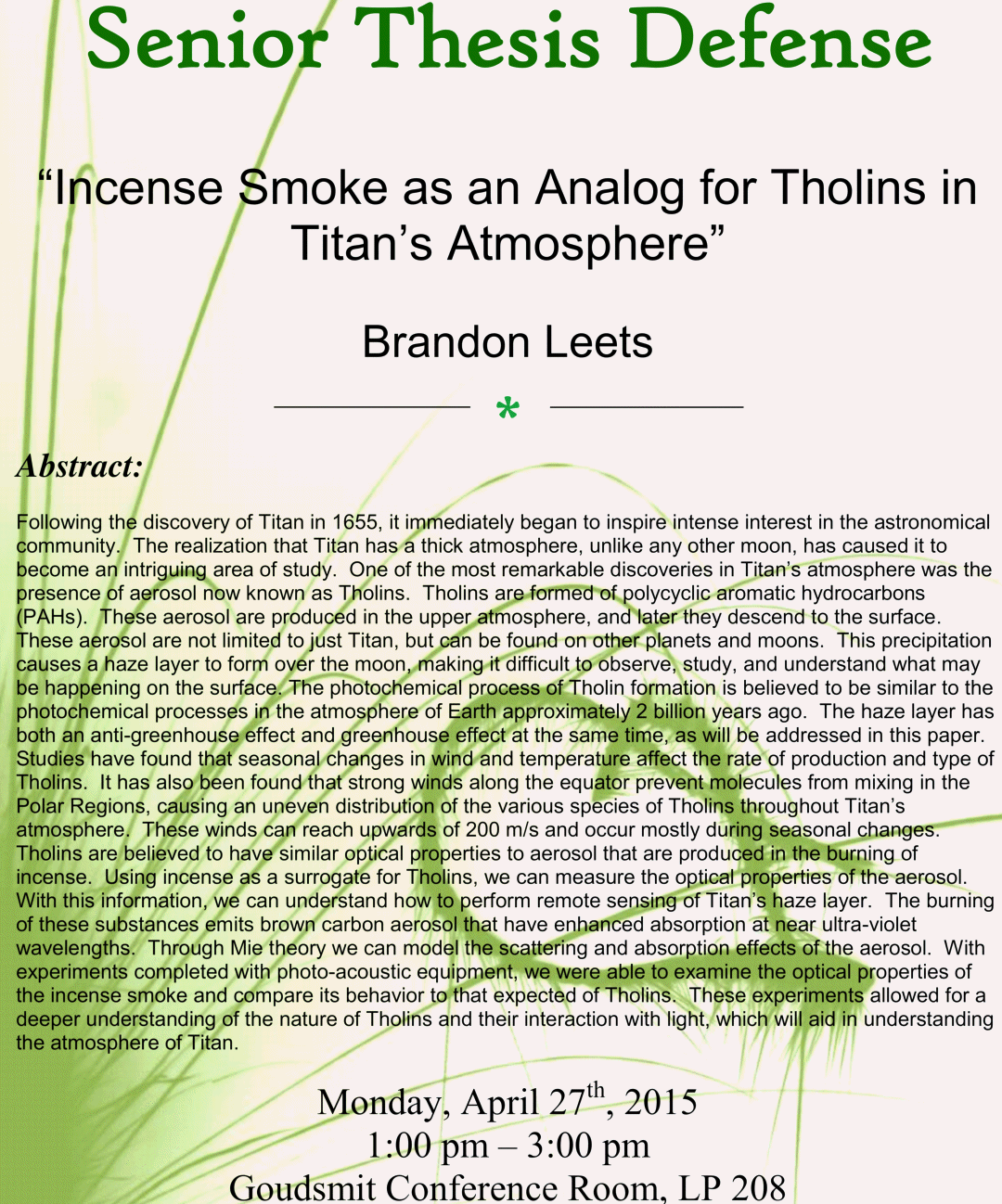
Here is announcement of a senior thesis defense with both Astronomy and Atmospheric Science connections.
You are welcomed and encouraged to attend if possible. All Physics and Atmospheric Science students are required to do a senior thesis project,
and this one can give you ideas about the sorts of topics and methods you might use.
Class on Tuesday: 7:30 am to 8:45 am in RM DMS 106 to work with the data from last Thursday.
Students will continue to work in groups as described in the Week 12 notes to analyze data and prepare their presentation.
As a group member it's important to do your part, to contribute to the overall success of the group. Each group will have a presentation.
Here's a generic outline for the presentation:
1. Introduction to that part of the campaign you worked on.
Discuss the science associated with your measurements.
2. Show a time series of your data (time on the x axis, and say pressure on the y axis if your group is responsible for the pressure measurements).l
3. Discuss how you did sensor calibration if necessary.
4. Discuss how your sensor works.
5. Intercompare sensor output with time series (for example, data from the UNR station and from the Teensy cards).
6. Discuss and interpret your data (for example, study the time evolution of the pressure and/or temperature for the Teensy card on the balloon sounding system).
7. Wrap up with suggestions for improving the experiment.
Class on Thursday: 8:00 am to 9:15 am in RM DMS 106 to work with the data from last Thursday with your group.
Week 12: 13 April
Class on Tuesday: 7:30 am to 8:45 am in RM DMS 106 to work with the data from last Thursday.
Class on Thursday: 8:00 am to 9:15 am in RM DMS 106 to work with the data from last Thursday with your group.
Here's the board notes for Tuesday (click on images for larger version).
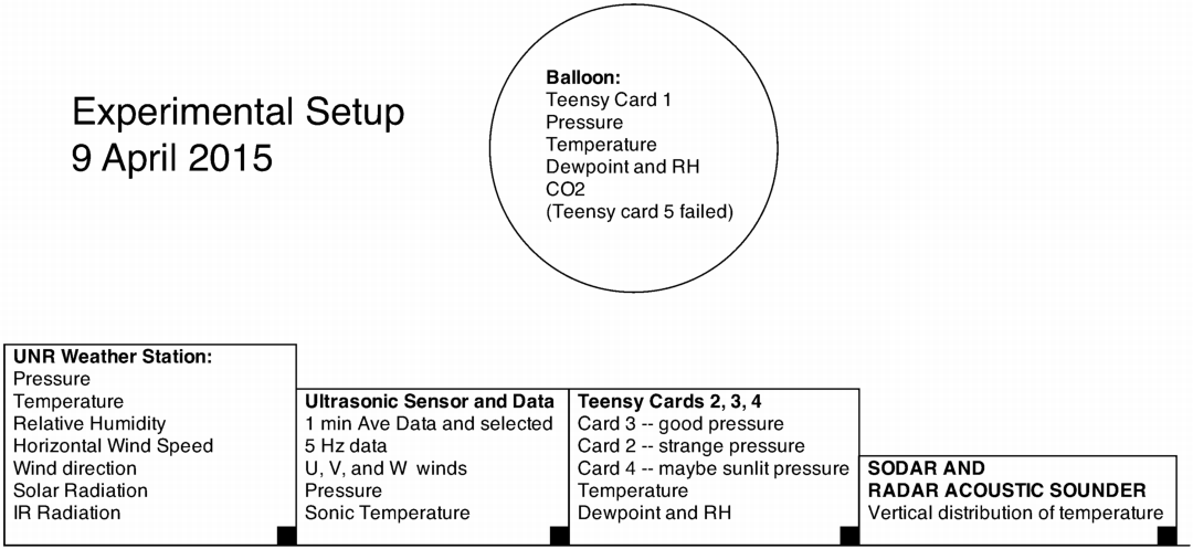
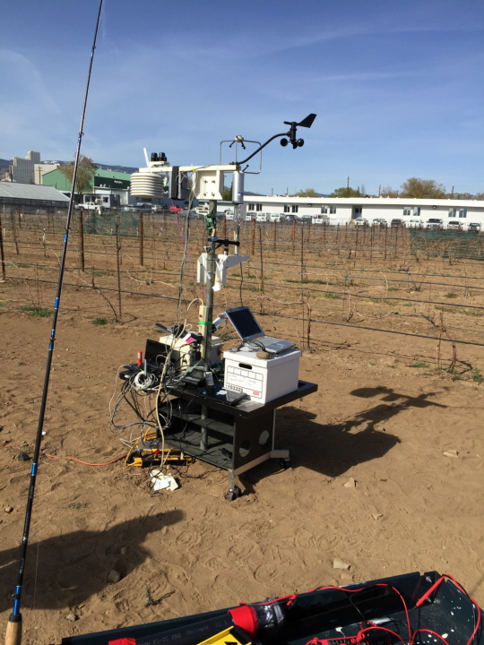
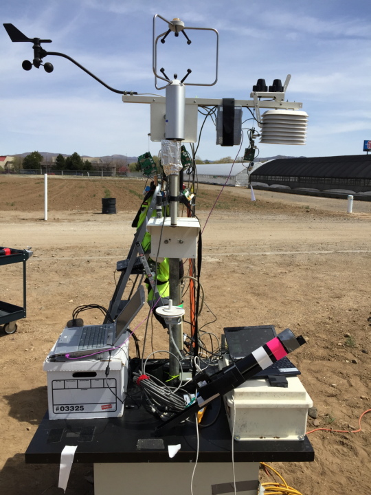
Here is the experimental set up we used on Thursday 9 April 2015. NOTE: the Sodar and Radar acoustic sounder also obtained vertical distribution of winds.
Group Assignments (tasks that need to be accomplished and prepared to discuss with a Powerpoint presentation):
Everyone should use the same time, UTC.
1. Pressure Group: (Zoey, Aaron, Jordan) Presentation
Calculate the time series of balloon altitude using calibrated Teensy Card 1 data and the hydrostatic equation.
Diagnose the reason(s) for Teensy cards 2, 4, and 5 to misbehave with pressure. (Card 5 probably just had poor power connection).
May need to acquire more data.
Diagnose and compare UNR weather station pressure with that of the Teensy card 3 for as long as possible (24 hours if possible, using large USB power supply).
Use the vertical distribution of Sodar and Radar Acoustic Sampler data to diagnose the pressure variations in the balloon sampler data.
2. CO2 group: (Samuel, Nick, Jasmine)
Compare CO2 measurements from Teensy cards 1 through 4. Calibrate the 'good ones' to a concentration average of 400 ppm for the time
interval 17:45:00 to 18:45:00 UTC. Report on the CO2 sensor readings for the day, especially the balloon sampler sensor, Teensy card 1. Here's the sketch used for the Teensy microcontroller acquisition of CO2 and its calibration.
You can download the windows USB driver for the Teensy to view its output with the Arduino IDE serial port monitor.
3. Temperature and Dewpoint Temperature group: (Chasity, Jason, Jessica)
Compare temperature and dewpoint temperature, and calibrate the Teensy cards, as necessary.
Use the UNR Weather Station Temperature and RH (turned into dewpoint temperature) as the calibration standard, and calibrate, as done for pressure,
for the time interval 17:45:00 to 18:45:00.
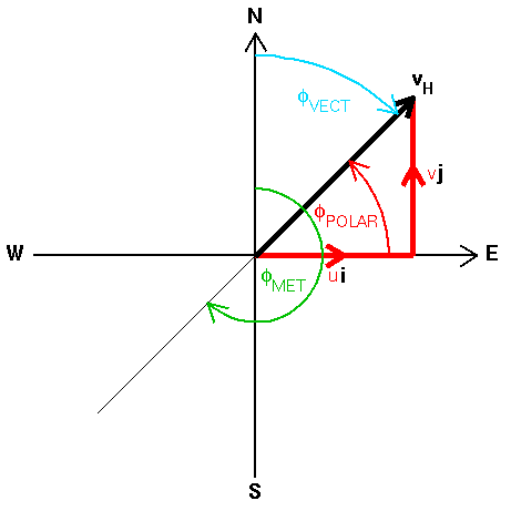
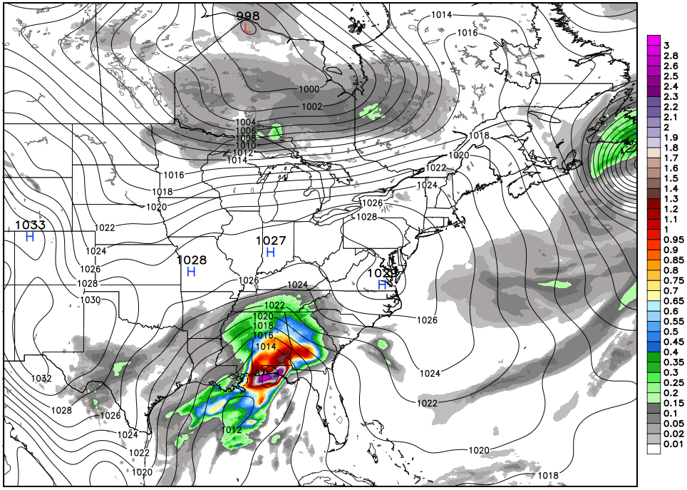
4. Wind and Synoptic Meteorology group: (Patricio, Marcelo, Kayla, Andrew)
Calculate the U and V components of wind from the UNR Weather Station, using the necessary trigonometry with wind direction and wind magnitude.
Calculate the 10 minute averaged U and V components of wind from the ultrasonic anemometer. Compare these. Also display and discuss the W component of wind from
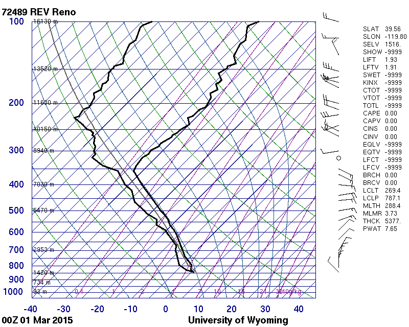
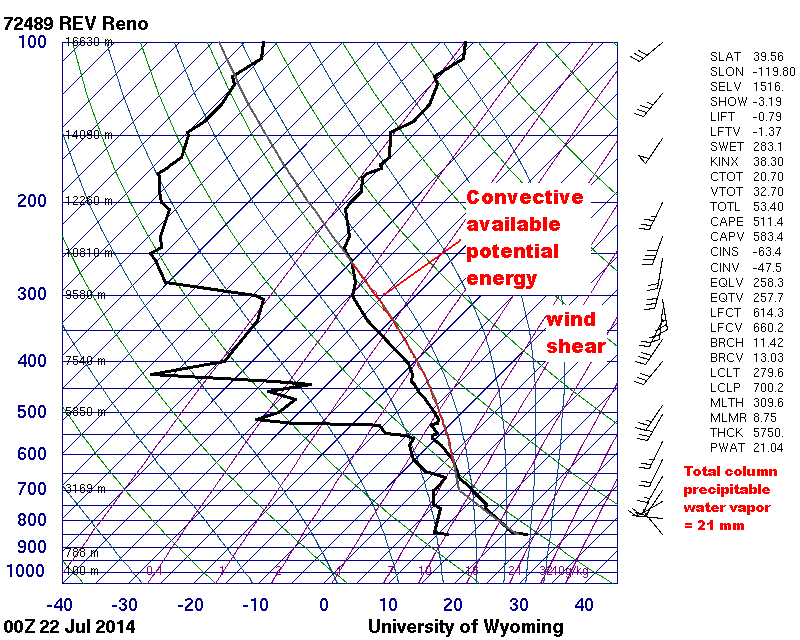
the ultrasonic anemometer, using the 1 minute averaged data. Acquire the National Weather Service balloons soundings for 12:00 UTC on April 9th and 00:00 UTC on April 10th and discuss
the reasons why we saw cirrus clouds that day (see below images.) Be sure to include frost point calculations when you request the soundings from the University of Wyoming site.
Discuss the overall weather trends we saw last week, leading up to Thursday, and the general locations of surface lows and highs, and upper level troughs, ridges, and jet streams.
5. Wind turbulence group: (Yunpeng, Thishan, Josette)
Discuss the derivation of, and measurements of, kinetic energy and turbulent kinetic energy during the measurement time. Check these
calculations by redoing them from the saved 5 Hz data (the ultrasonic data labeled as 'RAW'). Do selected time series graphs in the early morning and afternoon, illustrating
the RAW U, V, and W winds compared with the 1 minute averaged U, V, and W winds.
IMAGES FROM THE MEASUREMENTS ON 9 APRIL 2015
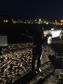
Early morning balloon launch.
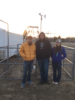
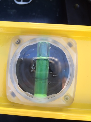
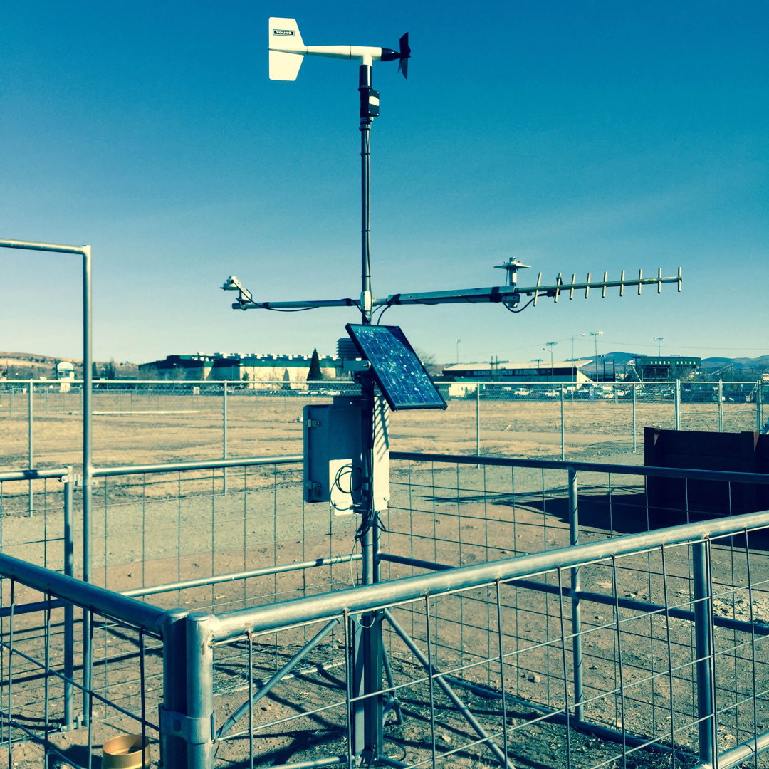
UNR weather station.
Ice crystals on level in the early morning.
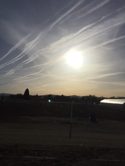
Contrails and cirrus clouds present
just after sunrise.
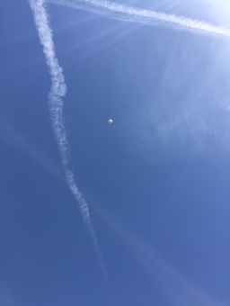
Balloon and contrails.
Setting up for measurements in the wee hours.
Ultrasonic anemometer and weather station.
Ultrasonic anemometer and weather station, another view.
Useful and Related Information:
The meteorological wind direction for this wind vector is about 225 degrees.
How to convert wind speed and meteorological direction to u and v components.
Week 11: 6 April
CLASS ON THURSDAY: EVERYONE WHO THAT WANTS TO GO TO THE WEATHER SITE DURING CLASS HOURS,
MEET AT THE CLASSROOM AT 7:45 A.M. WADE CLINE WILL WALK WITH STUDENTS TO THE SITE.
OTHERWISE, IF YOU WISH TO VISIT AT ANOTHER TIME UP TO 2 P.M., FOLLOW THE INSTRUCTIONS BELOW.
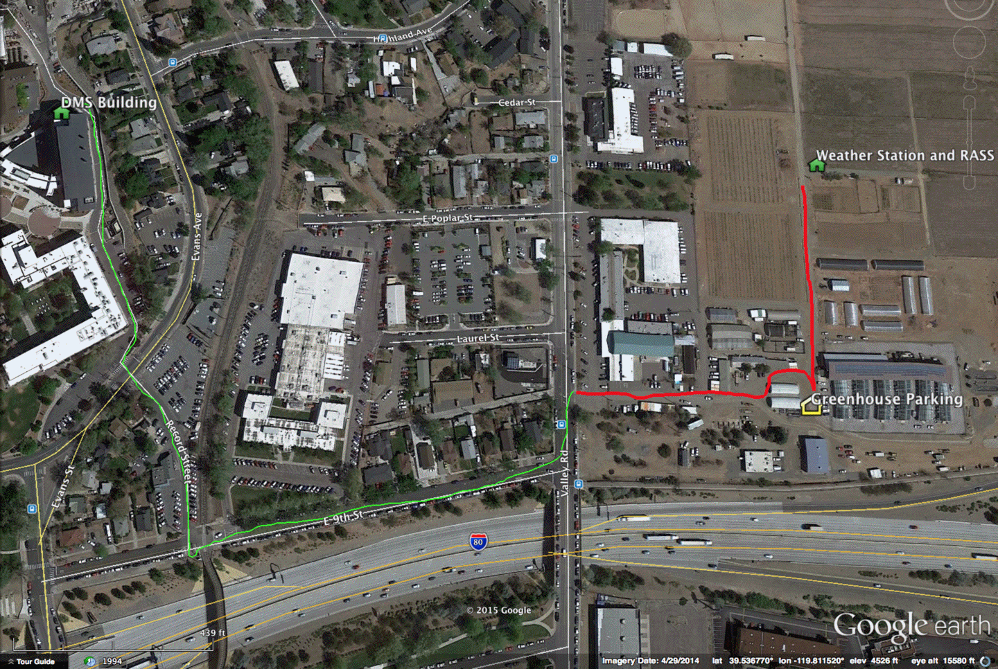
We will meet at the weather station on Valley Road for measurements. The walking path is shown in green (to get to the gate).
If necessary, you can probably to the Greenhouse location, and park near the greenhouse.
The assignment is to visit the weather station between 5 a.m. and 2 p.m.
Bring your camera (cell phone or otherwise) if you have one and get images of the sensors.
Document the ultrasonic anemometer for wind measurement, the balloon sounding system,
the standard weather station, and the class weather station based on the microcontroller that is used on the balloon system.
Also observe the radar acoustic sounding system and the UNR weather station. Identify the sensors on the UNR weather station.
We will do measurements of the atmosphere on Thursday, and this will be a case study for us to analyze. We will compare the wind direction and speed
measurements from the weather stations, will document the wind kinetic energy and turbulent kinetic energy in the still of the morning and in the afternoon,
and will look at the vertical distribution of temperature, humidity, and carbon dioxide concentration using the balloon sampling system.
This day will become a case study for us.
Here's the map for getting to the measurement location. The walking path from the DMS building is show in green, to the vicinity of the greenhouse.
The red path shows the path on site.
Class on Tuesday: 7:30 am to 8:45 am in RM DMS 106 Most Likely, But Check Back On Monday.
Here are the instructions for students using the Arduino based digital IR sensor over the weekend. Let me know if you have problems.
WINDOWS VERSION
Here is an executable software package to use the sensor with Ardunio and Labview to visualize the temperature sensor output. This is the windows version of the executable to be used for those that checked out an Arduino kit for the weekend to do measurements of the atmosphere over this time.
MACINTOSH VERSION (Includes detailed instructions)
Here is an executable software package to use the sensor with Ardunio and Labview to visualize the temperature sensor output. This is the Macintosh version of the executable to be used for those that checked out an Arduino kit for the weekend to do measurements of the atmosphere over this time.
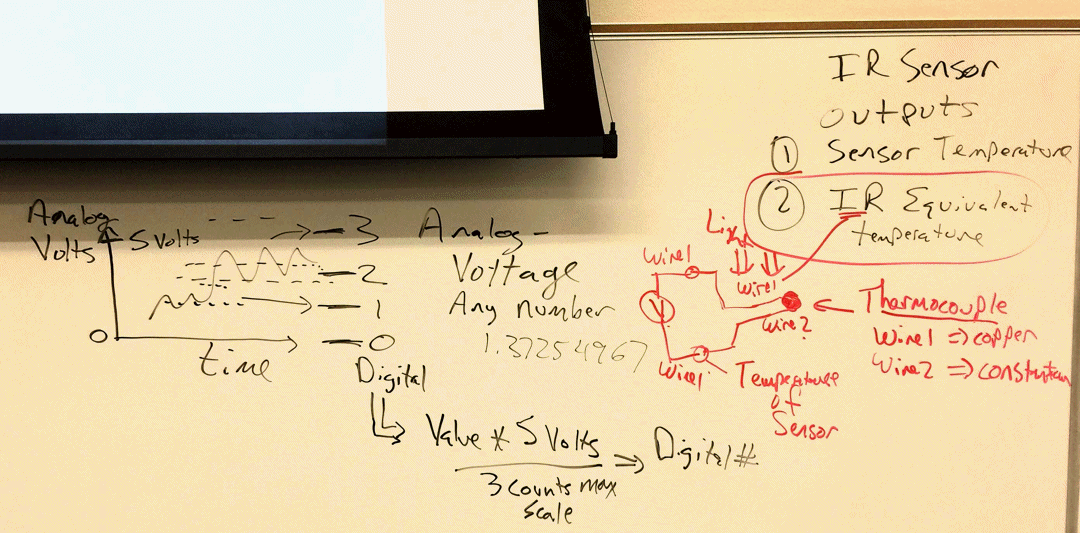
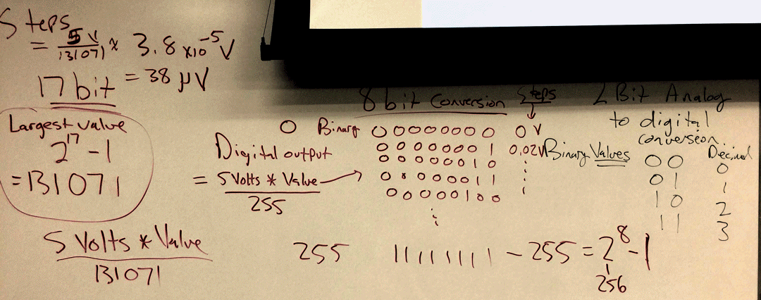
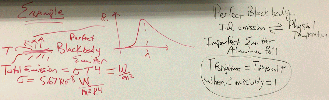
Here's the schematic of a IR sensor, from here.
The silicon filter passes IR radiation.
The blackbody absorbs IR radiation and heats up.
A thermopile (thermocouples connected in series) is below the blackbody; it provides a small voltage, perhaps microvolts.
The thermistor measures the overall chip temperature, and that is the thermopile reference junction temperature.
Week 9: 23 March
Class on Tuesday: 7:30 am to 8:45 am in RM DMS 106.
We will finish up the lab work for the LED and Arduino introduction.
Assignment 4, be sure you get all of your data by the end of class on Thursday.
Be sure you have as much of it done as possible for class on Tuesday.
Bring questions to class.
Class on Thursday: 8:00 am to 9:15 am in RM DMS 106.
Notes from last week as a review.
We will continue to work with breadboarding and use of digital volt meters.
The next assignment will be on LEDs.
Here is the framework for the next assignment.
We will continue to work with breadboarding and use of digital volt meters.
The next assignment will be on LEDs.
Here is the framework for the next assignment.
Here is the board from Thursday's class. Click on the images for a larger version.
Class on Tuesday: 7:30 am to 8:45 am in RM DMS 106.
Last Thursday we developed a case study for June 1st 2012 AERONET data analysis, showing the AOD over Reno as measured with the UNR Cimel
sunphotometer. We went through HYSPLIT back trajectory analysis. We developed the basic requirements for this homework assignment
as given here. Write a paragraph on each of the questions posed in the homework assignment description.
Here is the board from Tuesday's class. Click on the images for a larger version.
Class on Tuesday: 7:30 am to 8:45 am in RM DMS 106.
Here's the developing report and what we worked on in class on Tuesday: (click on image for larger version)
We began use of HYSPLIT back trajectory analysis for this mini case study.
PHYSICS DEPARTMENT COORDINATES FOR THE AERONET STATION AT UNR:
39.5410239 N = 39 degrees 32 minutes, 27.6864 seconds
119.8142892
W = 119 degrees 48 minutes 51.4404 seconds
Class on Thursday Meets: 8:00 am to 9:15 am in RM DMS 106.
Assignment 3 has been posted. We will look at the King Fire case study to prepare for this assignment.
First Topic: Look at the 1 June 2012 UNR AERONET AOD and do back trajectory analysis for 17 Z and 21 Z.
Our next module will be to learn how to use the HYSPLIT model (<<--- read this introduction) for air trajectories as part of meteorological analysis for air pollution and meteorological events interpretation and forecast.
We ask the questions, where did that wind come from? Where is it going?
Case study of the King fire smoke plume, 16 September 2014.
UNR Cimel sunphotometer showing a short pulse of smoke at 2 pm PDT and the main plume starting to arrive at
4 pm on the 16th. Click on image for a larger version. Data from NASA AERONET.
Image of the sky looking west from the Physics building at 1:53 pm. The leading edge smoke is very 'white', likely from smoldering fire, while the browner, thicker part closer to the horizon it likely due to intense flaming fire conditions. It likely contains brown carbon aerosol (enhanced absorption at shorter wavelengths). Click for larger image.
Image of the sky later, 5:13 pm PDT, after the second pulse of smoke had arrived. West Reno is not visible anymore. A contrail passes under the sun. Click on the image for a larber version.
Image of the sky at 5:32 pm PDT, showing a colorful sundog on the right due to cirrus clouds and some altocumulus clouds. Total optical depth is from gases, aerosol, and clouds. Click on image for a larger version.
MODIS instrument aboard NASA Terra satellite captured this image of the fire plume at 12:15pm PDT on 16 Sept 2014. Click on the image for a larger size.
MODIS instrument aboard NASA Aqua satellite captured this image of the fire plume at 1:55pm PDT on 16 Sept 2014 as the first pulse of white smoke reached Reno. Click on the image for a larger size.
King fire PM 2.5, black carbon, and brown carbon mass concentration estimated from the photoacoustic instruments at UNR Physics. PM2.5 was obtained from Bsca(532nm)/3.8 m^2/gram. BC from Babs(870 nm) / 5.38 m^2/gram. Brown carbon from Babs(405 nm)/11.56m^2/gram - BC. Click on the image for a larger size graph. Most of the aerosol is organic carbon. See this publication for a discussion.
Hysplit forecast trajectories showing smoke arriving in Reno around 4 pm local time on the 16th of September. Click on image for a larger version.
Class on Tuesday: 7:30 am to 8:45 am in RM DMS 106.
Spreadsheet we worked on to obtain 24 hour average data for the DRI weather station. Summary document that compares the meteorology at the DRI and UNR weather stations for July 2015.
Assignment 1 revision option was discussed. Students are encouraged to make an appointment at the UNR writing center as they prepare their revision.
Summary from Assignment 1. Click on images for larger view.
Class on Thursday Meets: 8:00 am to 9:15 am in RM DMS 106.
Board notes on aerosol, spectroscopy, optical depth, and the atmosphere.
Assignment 3 has been posted. We will look at the King Fire case study to prepare for this assignment.
Our next module will be to learn how to use the HYSPLIT model (<<--- read this introduction) for air trajectories as part of meteorological analysis for air pollution and meteorological events interpretation and forecast.
We ask the questions, where did that wind come from? Where is it going?
Case study of the King fire smoke plume, 16 September 2014.
UNR Cimel sunphotometer showing a short pulse of smoke at 2 pm PDT and the main plume starting to arrive at
4 pm on the 16th. Click on image for a larger version. Data from NASA AERONET.
Image of the sky looking west from the Physics building at 1:53 pm. The leading edge smoke is very 'white', likely from smoldering fire, while the browner, thicker part closer to the horizon it likely due to intense flaming fire conditions. It likely contains brown carbon aerosol (enhanced absorption at shorter wavelengths). Click for larger image.
Image of the sky later, 5:13 pm PDT, after the second pulse of smoke had arrived. West Reno is not visible anymore. A contrail passes under the sun. Click on the image for a larber version.
Image of the sky at 5:32 pm PDT, showing a colorful sundog on the right due to cirrus clouds and some altocumulus clouds. Total optical depth is from gases, aerosol, and clouds. Click on image for a larger version.
MODIS instrument aboard NASA Terra satellite captured this image of the fire plume at 12:15pm PDT on 16 Sept 2014. Click on the image for a larger size.
MODIS instrument aboard NASA Aqua satellite captured this image of the fire plume at 1:55pm PDT on 16 Sept 2014 as the first pulse of white smoke reached Reno. Click on the image for a larger size.
King fire PM 2.5, black carbon, and brown carbon mass concentration estimated from the photoacoustic instruments at UNR Physics. PM2.5 was obtained from Bsca(532nm)/3.8 m^2/gram. BC from Babs(870 nm) / 5.38 m^2/gram. Brown carbon from Babs(405 nm)/11.56m^2/gram - BC. Click on the image for a larger size graph. Most of the aerosol is organic carbon. See this publication for a discussion.
Hysplit forecast trajectories showing smoke arriving in Reno around 4 pm local time on the 16th of September. Click on image for a larger version.
Useful and Related Information:
Figure 1. Timelapse video showing the UNR Cimel sunphotometer in operation as part of NASA's AERONET network of
sunphotometers used to evaluate satellite retrieval algorithms and to characterize the local atmosphere.
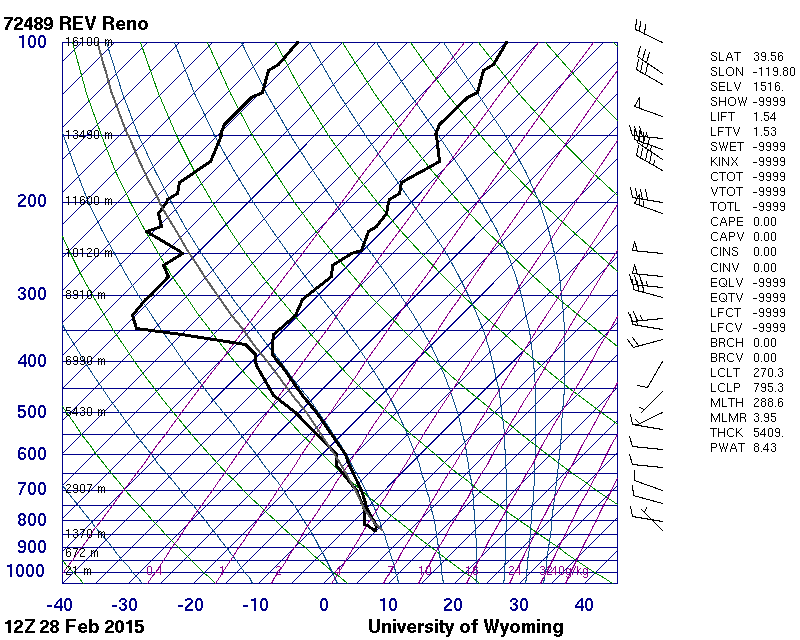
Our next module will be to look at the balloon soundings from the Reno National Weather Service another way of learning about the thermodynamics of the atmosphere.
We will study the skew T logP thermodynamic diagram. Here is a blank copy of the skew T to use (click on the image to bring up a larger version that can be printed for high resolution).
Bring your draft of Assignment 1 to class on Thursday.
Here's what we worked on during Tuesday's class:
(Added a histogram of lapse rate to the spreadsheet)
(prepared a quick template for the MSword document for assignment 1)
By Tuesday you should have most of the assignment 1 completed as homework. Refer to the assignment page.
You should have the month of July analyzed in the same way that we have analyzer the month of December.
Be sure you adequately copy and paste your figures into MSword for preparing the assignment. We will review this on
Tuesday as well. Class on Tuesday: 7:30 am to 8:45 am in RM DMS 106.
We'll meet in RM DMS 106 (computer room in the Davidson Math and Science Building). We'll continue from last week.
Class on Thursday Meets: 8:00 am to 9:15 am in RM DMS 106.
Here is the powerpoint presentation we developed in class to look at the balloon soundings on 5 February 2015.
Our next module will be to look at the balloon soundings from the Reno National Weather Service another way of learning about the thermodynamics of the atmosphere.
We will study the skew T logP thermodynamic diagram. Here is a blank copy of the skew T to use (click on the image to bring up a larger version that can be printed for high resolution).
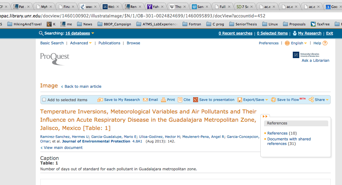
Here is the path we used to go to the UNR library website to find articles related to atmospheric temperature inversions.
Figure 1. Go to this website, and put in your search request. In this case the search request was "meteorological temperature inversions'.
Figure 2. Search outcome. We clicked on "Full Text Online" to bring up the image shown in Figure 3.
Figure 3. Result when clicking on "Full Text Online" in Figure 2. To get the article, click on "Export" and export it as a PDF document. That should put the article in your
downloads folder so you can read it and reference it if appropriate.
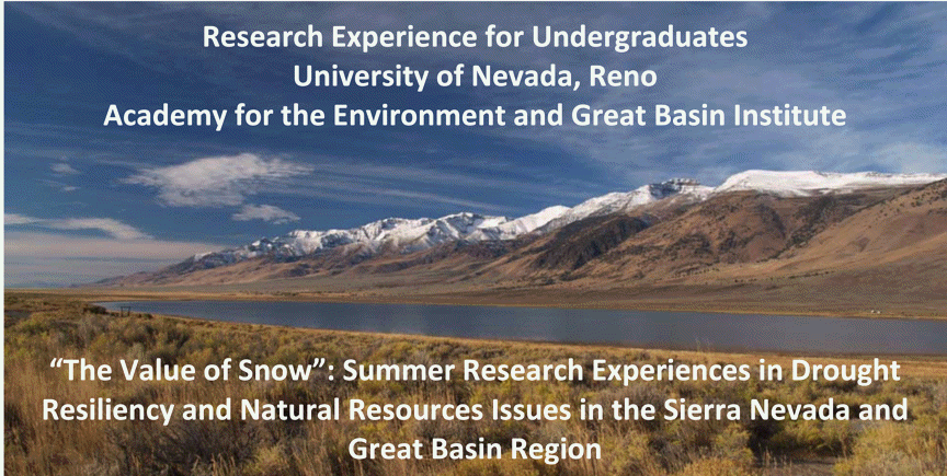
Here is an announcement of a local summer research program within the University of Nevada system. Details are at this link.
Week 2: 26 January
Class on Thursday Meets: 8:00 am to 9:15 am in RM DMS 106.
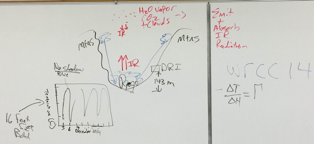
Here's the whiteboard notes.
NOTE THE NEW TIME FOR MEETING ON TUESDAY!
Class on Tuesday: 7:30 am to 8:45 am in RM DMS 106.
We'll meet in RM DMS 106 (computer room in the Davidson Math and Science Building). We'll continue from last week.
Class on Thursday: We'll meet in RM DMS 106 (computer room in the Davidson Math and Science Building). We'll work with the surface based meteorological data from the DRI weather stations in our area.
All of the Western Regional Climate Center Weather Sites
Look at site locations in Google Earth. Calculate elevation difference between the sites in km.
Download data from the UNR site for December 2014.
a. Plot a time series of temperature for this station.
b. Plot solar radiation as an overlay.
c. Plot IR radiation as an overlay.
d. Interpret.
Download data from the DRI site for December 2014 onto the same sheet.
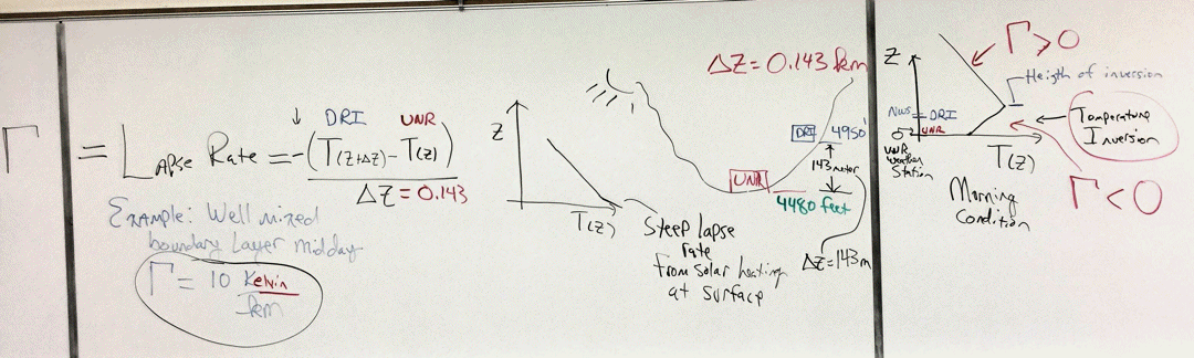
a. Calculate the negative temperature gradient (i.e. the lapse rate) in Kelvin / km (compare with the adiabatic lapse rate).
b. Overlay lapse rate with wind speed from both stations.
c. Interpret.
Outcome Thursday:
We worked with the UNR weather station data.
The topic is to evaluate temperature inversions in the morning in Reno.
Keep working with excel to achieve the desired graphical format, and bring your spread sheet to class on Tuesday.
UNR Weather station image. Click on image for a larger version.
Notes from board during class on Thursday. Click on image for larger version.
 Balloon and contrails.
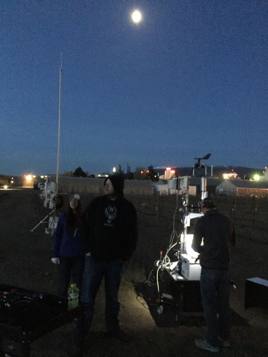


 SCL pin


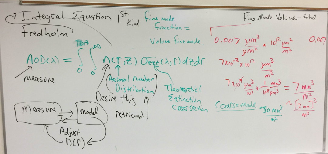
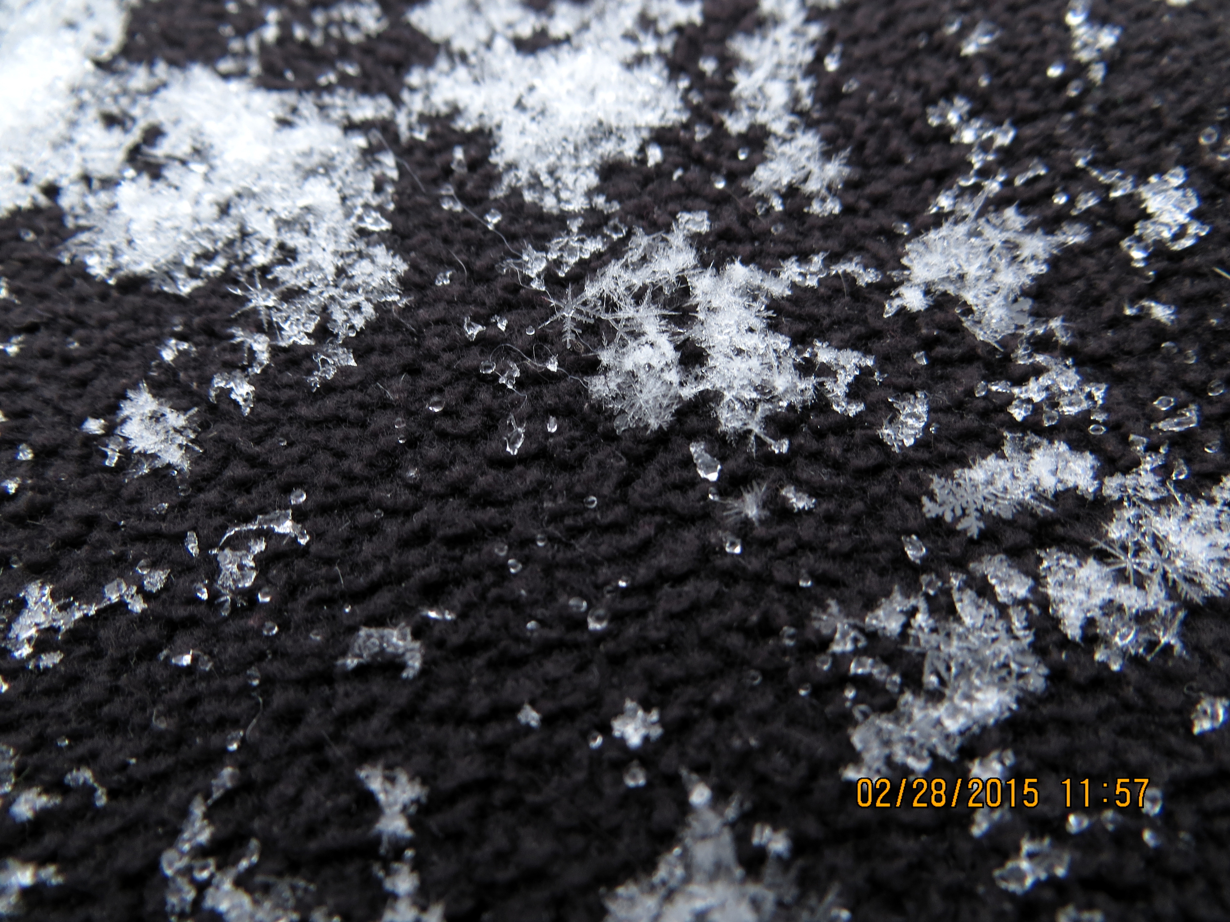
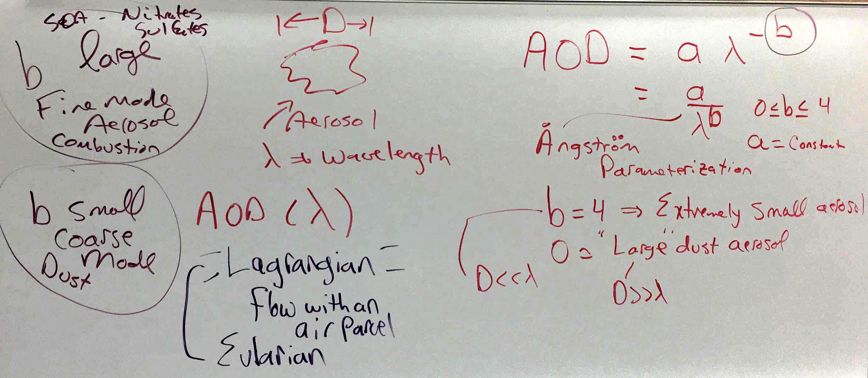
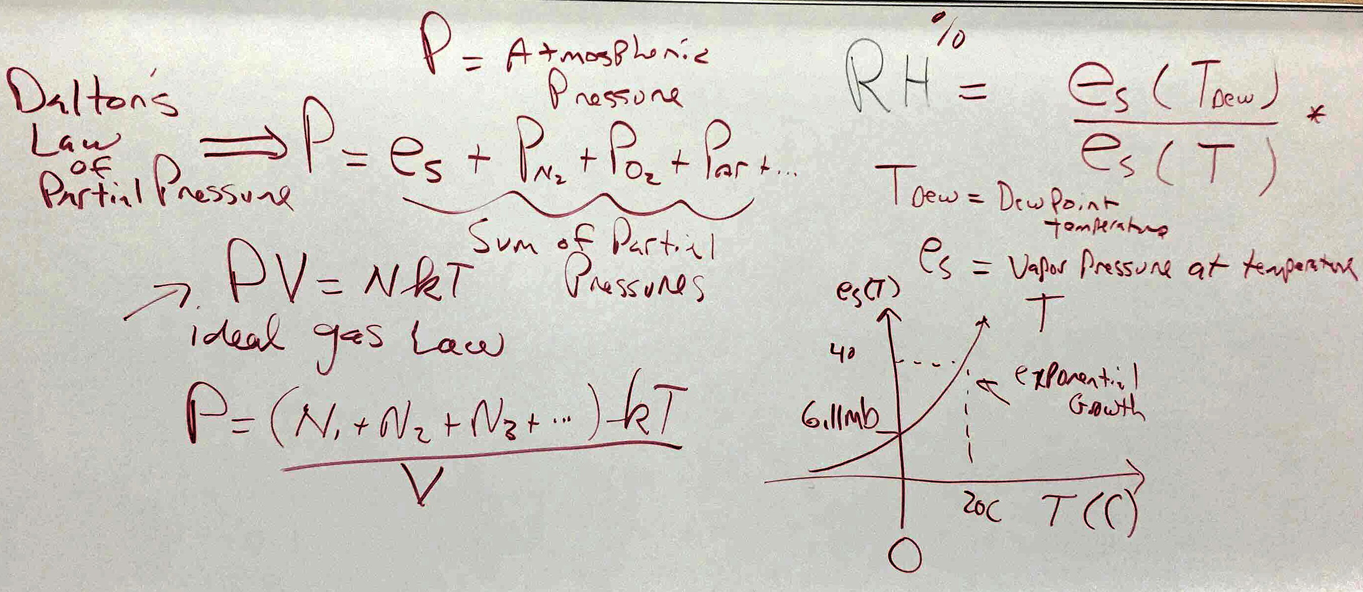
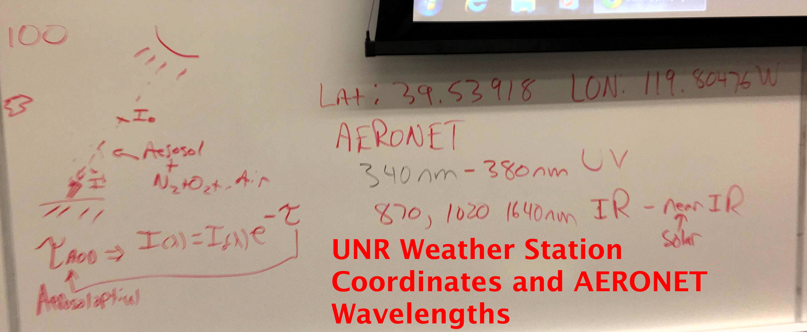
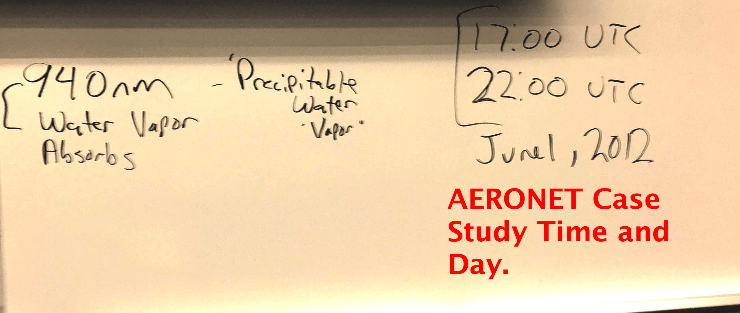
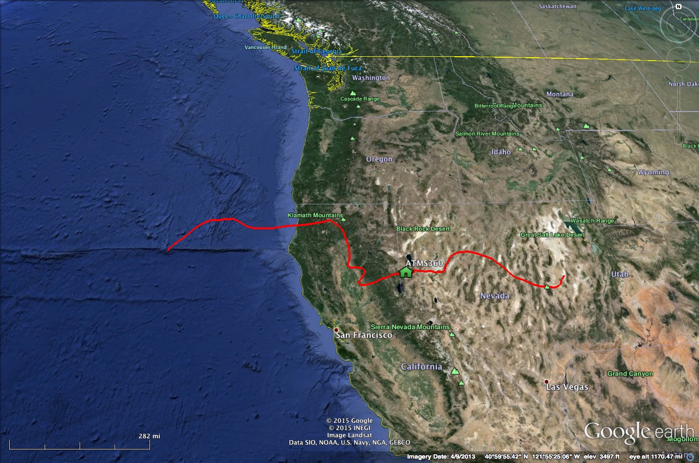


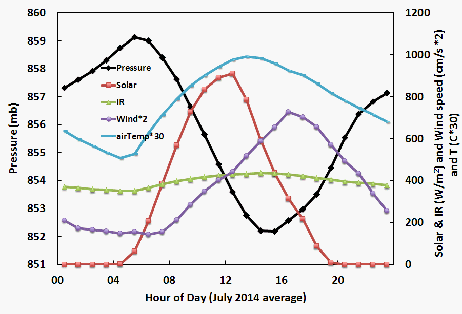
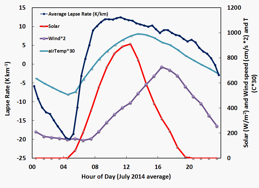
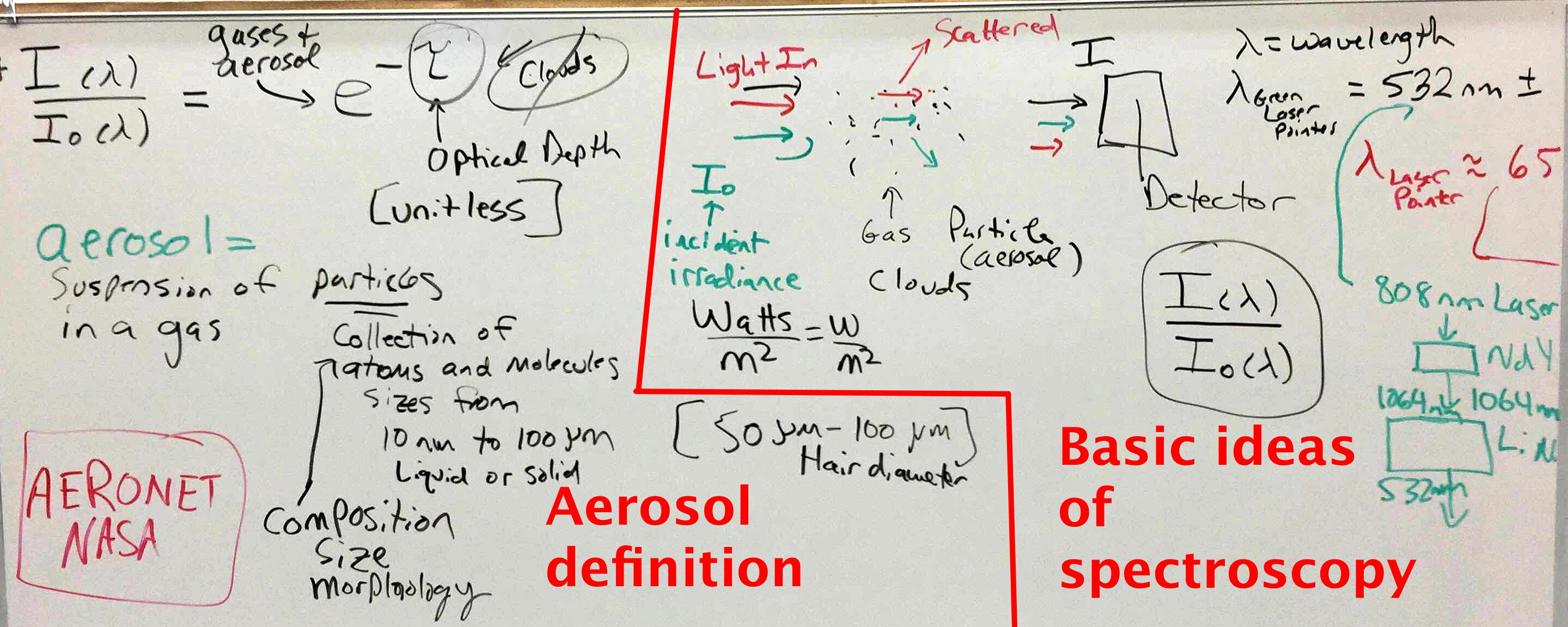
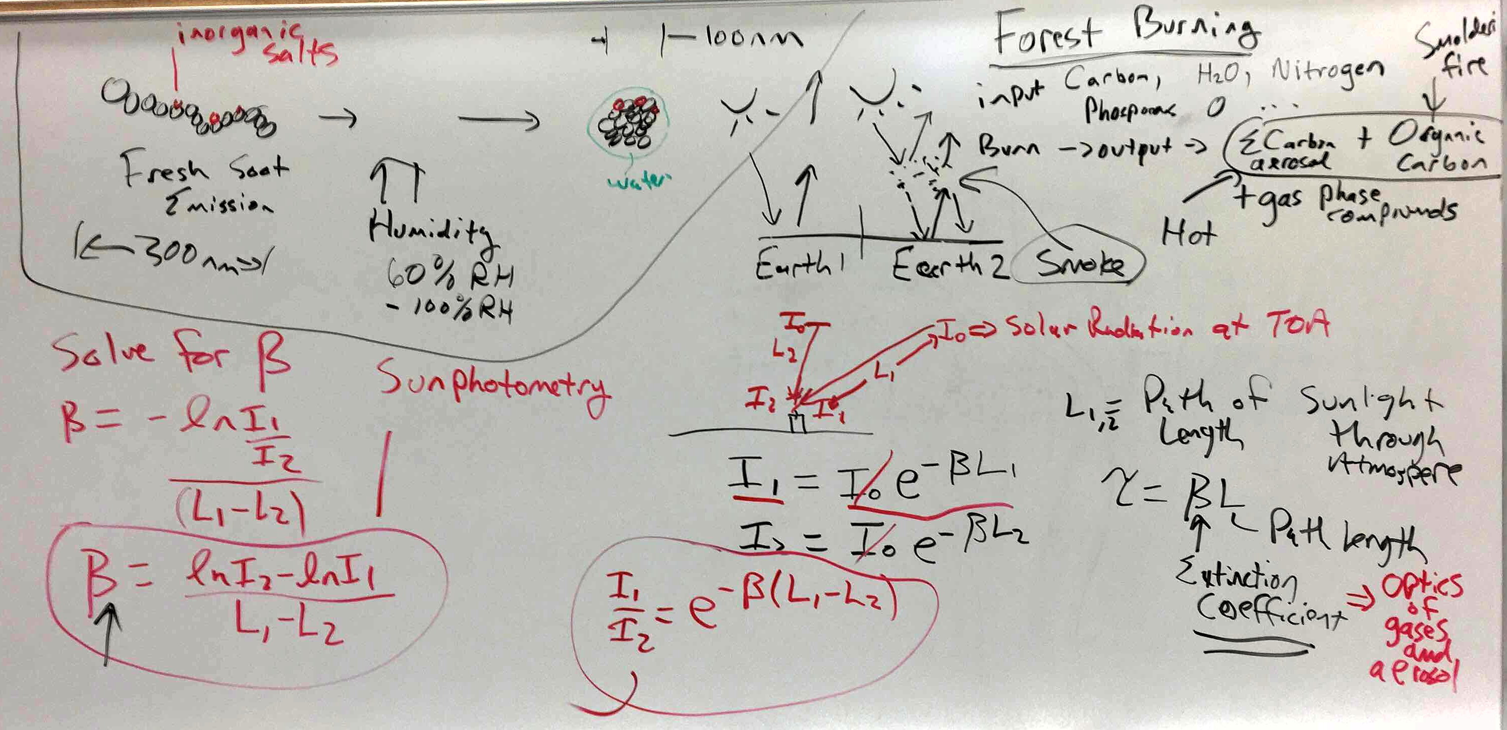
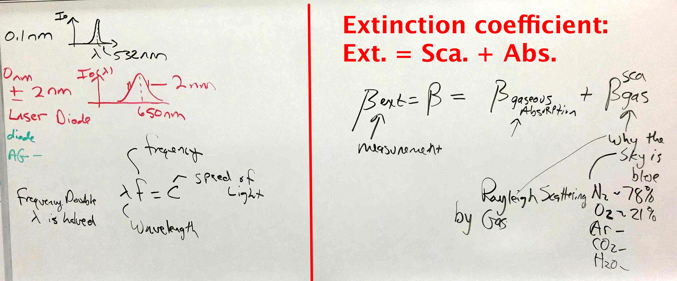
 Figure 2. Weather image (and see discussion) from the
 Undergraduate Summer Research Opportunity (